Odds Ratio confidence interval

When performing logistic regression, epidemiologists and other researchers are usually interested in the Odds Ratio (OR) estimates rather than the regression coefficients. As we all know, OR is esimated by exp(beta estimate). Most statitical software provide beta estimates, alog with the stndard errors of these estimates, and usually a confidence interval for beta is beta plus/minus 1.96SE(beta).
A confidence interval for the OR is howevr more tricky. Some references adise to o take the CI for beta and just exponent it, so a CI for the OR would be exp[beta plus/minus 1.96
SE(beta)]. This method has a nice property: if the CI for beta does not contain zero, so the exponented CI does not contain Y. This is how SPSS, for example, calculates a CI for the OR.

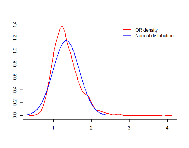
A different approch is to apply the delta method. When applying the method one gets that
SE(exp(beta))=SE(OR)=se(beta)OR
So a CI for OR would be OR +/- 1.96
se(beta)*OR

However: 1) It is possible that the lower CI will be negative. 2) It is possible that although the CI for beta does not contain zero, this CI will contain 1.
Apparently, epidemiologists think that this is a problem.
As a statistician, I do not see any problem, and my recommendation is to use the delta method. But… what would you recommend? and if you favor the delta method, how would you cummunicate this?

Fascinating. Errors for OR are generally not normally distributed so is this second approach “correct”?

Interesting. I mostly work in the Bayesian framework via mcmc and the approach there is just to exponentiate the log odds ratio at every step of the chain. This would be equivalent to option 1 in the case of flat priors and normally distributed log odds ratios.

I think option 1 assumes that log odds ratios are normally distributed, not odds ratios.

1 Like

Agree @timdisher!

Seems to me applying a non-linear transform to an estimate (e.g. beta) with normally distributed errors will result in non-normally distributed errors and violation of the concept of +/- 1.96 SD tor the CI…

1 Like

You may find this Stata FAQ helpful (even if you do not use Stata). Here is an excerpt:

To continue with the point that confidence intervals can be computed in two ways for transformed estimates (ORs, RRRs, IRRs, HRs, …), a user asked

Wouldn’t it be more appropriate to use the the standard errors for the RR when calculating CI?

Asymptotically, both methods are equally valid, but it is better to start with the CI in the metric in which the estimates are closer to normal and then transform its endpoints. Since the estimate b is likely to be more normal than exp(b) (since exp(b) is likely to be skewed), it is better to transform the endpoints of the CI for b to produce a CI for exp(b).

HTH.

1 Like

Have you tried a quick simulation study? I suspect that the Wald / delta method will not have the best properties.

This website mentions 8 methods:

2 Likes

I did the following quick simulation study in R. I think I did it right, but just in case the code is attached for review.

The delta method is giving me 0.9 coverage whereas the exponent version is returning the correct 0.95. The delta method appears to overly optimistic at these settings. I however tried various settings and for some ranges where the values were closer the coverage for the delta was good, the exponent version I never saw it vary.

p1 <- 0.9
p2 <- 0.1
n <- 100

truth <- (p2/(1-p2))/ (p1/(1-p1))

simulationDelta <- function()
{
x <- rbinom(n, 1, p1)
y <- rbinom(n, 1, p2)
data <- data.frame(group=rep(c(‘a’,‘b’), each=n), disease=c(x,y))
model <- glm(disease ~ group, data=data, family=binomial)
est <- exp(coef(model)[2])
se <- summary(model)$coefficients[2,2]
lci <- est - 1.96 * se * est
uci <- est + 1.96 * se * est

(lci <= truth) && (uci >= truth)
}

studyDelta <- replicate(6000, simulationDelta() )
mean(studyDelta)

simulationExp <- function()
{
x <- rbinom(n, 1, p1)
y <- rbinom(n, 1, p2)
data <- data.frame(group=rep(c(‘a’,‘b’), each=n), disease=c(x,y))
model <- glm(disease ~ group, data=data, family=binomial)
est <- exp(coef(model)[2])
se <- summary(model)$coefficients[2,2]
lci <- exp(coef(model)[2] - 1.96 * se)
uci <- exp(coef(model)[2] + 1.96 * se)

(lci <= truth) && (uci >= truth)
}

studyExp <- replicate(6000, simulationExp() )
mean(studyExp)

3 Likes

When computing non-coverage probabilities always compute two of them, one for each tail. This will expose even more serious problems for the delta method.

4 Likes

When we are in the context of logistic regression, beta_hat, the estimator for the true regression coeficient beta of as independent variable X, is a maximum likelihod estimator, and therefore is assimptotically normal. Therefore the delta metod can be used to derive a normal-based confidence interval for exp(beta_hat), which is a maximum likelihood estimae for exp(beta), which is interpreted as the odds ratio of X with repect to the dependent variable Y.

Well, what does [quote=“bweaver, post:5, topic:1313”]
Asymptotically, both methods are equally valid
[/quote] mean? assimpoticaly, both ends of both CIs will approach the the true OR as the sample size approaches infinity. This is a nice theoretical result, but in prectice your sample size is always finite, so the the non asymptotic case is the interesting one. And here is the heart of the matter: it is possible that one of the confidence intervals will contain 1 while the other one does not. So one method leads you to non signifcant reult (and no publication :frowning: ) while the other one is statistically significant. So what would you do?

1 Like

And one more thing: The FAQ you refered to states that “When ORs (or HRs, or IRRs, or RRRs) are reported, Stata uses the delta rule to derive an estimate of the standard error of ORb”, despite the statement that “it is better to transform the endpoints of the CI for b to produce a CI for exp(b)” later in the same FAQ. So the question remains

I think we’re moving off point a bit. I don’t think Stata uses the standard error of the OR for anything. Its use is questionable because any valid confidence interval for OR must be asymmetric. And as you said asymptotic normality is not helping us in real data situations. That’s why we need to compute CIs on the best basis possible, i.e,. if we want to use a method that assumes symmetry we need to compute the standard error on a basis that is symmetric. More accurate: likelihood profile confidence intervals for ORs which will be properly asymmetric.

Please edit earlier posts rather that putting out consecutive posts. Thanks.

2 Likes

Thank you for the link. However it refers to 2x2 tables, that are special cases of logistic regression with a single independent variable X which is categorical and have only 2 possible values. Second, I did a quick simulation study, and found that the difference between the distribution of exp(beta_hat) and the normal distribution is not unacceptable (this was done for a sample size of 100).

The code is:
simlogitistic=function(sample_size, alpha, beta, scale=1){

sim_results=list()
sim_results$sample_size=sample_size
sim_results$alpha=alpha
sim_results$beta=beta
sim_results$scale=scale

eps=rlogis(sample_size, 0, scale)
x=rnorm(sample_size)
y=as.numeric(alpha+beta*x+eps>0)
dat=data.frame(y,x)

model=glm(y~x, data=dat, family=binomial(link=“logit”))

msm <- as.numeric(suppressMessages(summary(model))$coefficients[2, 1:2])
estimate=msm[1]
estimate_se=msm[2]
sim_results$estimate=estimate
sim_results$estimate_se=estimate_se
return(sim_results)
}

sample_size=100
alpha=1
beta=0.25
scale=1
sim_results=data.frame(sample_size, alpha, beta, scale)

for(j in 1:1000){
sim_results[j,1:4]=c(sample_size, alpha, beta, scale)
testrun=simlogitistic(100,1,0.25,1)
sim_results$estimate[j]=testrun$estimate
sim_results$se[j]=testrun$estimate_se
}

sim_results$exp_estimate=exp(sim_results$estimate)
exp_estimate_mean=mean(sim_results$exp_estimate)
exp_estimate_mean_std=sqrt(var(sim_results$exp_estimate))

d=density(sim_results$exp_estimate)

L=exp_estimate_mean-3exp_estimate_mean_std
W=6
exp_estimate_mean_std
step=W/100
q=L+step*0:100
plot(density(sim_results$exp_estimate), col=“red”, lwd=2, pch=0.8,
main=title, xlab=“OR”)
lines(q, dnorm(q, mean=exp_estimate_mean, sd=exp_estimate_mean_std),
col=“blue”, lwd=2, pch=0.8)
legend(x=“topright”, box.lty=0, col=c(“red”, “blue”),
legend=c(“OR density”, “Normal distribution”),
lwd=2, inset=c(0.01,0.01))

You’re beating a dead horse. Not unacceptable? Both tails are wrong. Compute the left and right non-coverage probabilities.

1 Like

Not sure I understand why is that. Are you also saying that a symetric CI for the OR will be invalid?

Frank is right, Stata does not use that (delta rule) SE to compute the CI for the OR. Here is a demo using the same data as in that FAQ, but using Stata’s -logit- command rather than -logistic-, because the output is a bit clearer, IMO.

. webuse lbw, clear
(Hosmer & Lemeshow data)

. logit low age lwt i.race smoke

Iteration 0:   log likelihood =   -117.336  
Iteration 1:   log likelihood = -107.52033  
Iteration 2:   log likelihood = -107.29661  
Iteration 3:   log likelihood = -107.29639  
Iteration 4:   log likelihood = -107.29639  

Logistic regression                             Number of obs     =        189
                                                LR chi2(5)        =      20.08
                                                Prob > chi2       =     0.0012
Log likelihood = -107.29639                     Pseudo R2         =     0.0856

------------------------------------------------------------------------------
         low |      Coef.   Std. Err.      z    P>|z|     [95% Conf. Interval]
-------------+----------------------------------------------------------------
         age |  -.0225071   .0341688    -0.66   0.510    -.0894766    .0444625
         lwt |  -.0125017   .0063843    -1.96   0.050    -.0250146    .0000113
             |
        race |
      black  |    1.23121   .5171062     2.38   0.017     .2177006    2.244719
      other  |   .9435946   .4162001     2.27   0.023     .1278573    1.759332
             |
       smoke |   1.054433   .3799787     2.77   0.006     .3096879    1.799177
       _cons |   .3301267   1.107607     0.30   0.766    -1.840743    2.500997
------------------------------------------------------------------------------

. matrix tab = r(table)'

. matrix list tab

tab[7,9]
                      b          se           z      pvalue          ll          ul
    low:age  -.02250707   .03416876  -.65870331   .51008631   -.0894766   .04446246
    low:lwt  -.01250169   .00638428  -1.9581978   .05020681  -.02501465   .00001128
low:1b.race           0           .           .           .           .           .
 low:2.race     1.23121   .51710617   2.3809618    .0172675   .21770056   2.2447195
 low:3.race   .94359458   .41620012   2.2671656   .02338011   .12785734   1.7593318
  low:smoke   1.0544326   .37997875   2.7749778   .00552055   .30968791   1.7991772
  low:_cons   .33012671   1.1076071   .29805398   .76566196  -1.8407433   2.5009968

                     df        crit       eform
    low:age           .    1.959964           0
    low:lwt           .    1.959964           0
low:1b.race           .    1.959964           0
 low:2.race           .    1.959964           0
 low:3.race           .    1.959964           0
  low:smoke           .    1.959964           0
  low:_cons           .    1.959964           0

. svmat tab

. generate double OR = exp(tab1)
(182 missing values generated)

. generate double ORSE = exp(tab1)*tab2
(183 missing values generated)

. generate double ORlower = exp(tab5)
(183 missing values generated)

. generate double ORupper = exp(tab6)
(183 missing values generated)

. list OR-ORupper if !missing(OR), clean noobs

           OR        ORSE     ORlower     ORupper  
    .97774432   .03340831   .91440965   1.0454657  
    .98757614   .00630496   .97529563   1.0000113  
            1           .           .           .  
    3.4253717   1.7712809   1.2432147   9.4377679  
       2.5692   1.0693013   1.1363909    5.808555  
    2.8703458   1.0906704   1.3629997   6.0446717  
    1.3911444   1.5408414   .15869942   12.194644  

. logit, or noheader
------------------------------------------------------------------------------
         low | Odds Ratio   Std. Err.      z    P>|z|     [95% Conf. Interval]
-------------+----------------------------------------------------------------
         age |   .9777443   .0334083    -0.66   0.510     .9144097    1.045466
         lwt |   .9875761    .006305    -1.96   0.050     .9752956    1.000011
             |
        race |
      black  |   3.425372   1.771281     2.38   0.017     1.243215    9.437768
      other  |     2.5692   1.069301     2.27   0.023     1.136391    5.808555
             |
       smoke |   2.870346    1.09067     2.77   0.006        1.363    6.044672
       _cons |   1.391144   1.540841     0.30   0.766     .1586994    12.19464
------------------------------------------------------------------------------
Note: _cons estimates baseline odds.

. 
end of do-file

Compare the CIs in the listing to those in the final table–they’re the same, and both were achieved by exponentiating the limits of the CI for B.

HTH.

1 Like

I don’t know, but I look at the table, and see that indeed the CI for the OR are calculated using by exponenting the CI for alpha. On the other hand, the Z test is calculated by using the delta method. So, if a symetric CI for the OR is invalid, how do you justify a symetric test on OR? And more: in this case everything is fine. CI contains 1, Z is not significant. But what would you do if you get a contradicting results?

I must admit I really don’t understand.
About right and wrong: both curves are right - they are calculated from the results of the simulation. They are not wrong unless you claim that the simulation and the following calculations are wrong. Are the red and blue curves suffciently close? this is debatable. The real question is whether you can use the blue line to produce a confidence interval with the desired confidence level, and the answer is that yes, you can. And it can be proved both mathematically, and empirically using suimulations.

Regarding the left and right non-coverage probabilities: why do they matter? When dealing with confidence intervals, what matters is the coverage probability, and both methods lead to a 95% coverage probability. Oh, and there is one more thing - a narrower confidence interval is better. It is easy to see that the delta method yields a narrower confidence interval when comparing it to the other method.

Don’t even contemplate getting the SE of an OR (or indeed a RR). Such quantities naturally behave on a ratio scale – not surprisingly – and the distribution on the original scale wouldn’t be remotely symmetrical. The resulting interval isn’t remotely boundary-respecting. The simplest approach is always to get a SE-based CI for log OR, then exponentiate the two limits.

HOWEVER – for most issues relating to proportions, SE-based methods go wrong, sooner or later. The snag usually relates to zero or near-zero cells. Here, if any of the 4 cells of the 2 by 2 table is zero, the standard error blows up and no interval can be calculated. Interval location – the balance of left and right non-coverage probabilities – is also an issue here, as someone has already pointed out. And often, the mean coverage is far lower than the nominal 1-alpha (which we normally set at 95%).

There are better methods available – though they are necessarily rather more complex, both conceptually and computationally. For simple odds ratios and ratios of proportions, derived from a simple 2 by 2 frequency table, the score intervals developed by Miettinen & Nurminen are as good as you’ll get. They aren’t closed form, they require a single depth of iteration. That’s not a problem – they can be programmed in MS Excel using a fixed number of interval bisections.

These and other related methods are explained in detail in my book Confidence Intervals for Proportions and Related Measures of Effect Size. This is available at http://www.crcpress.com/product/isbn/9781439812785

A zip file K10649.zip is freely downloadable from this site. It contains a spreadsheet ODDSRATIOANDRR.xlsx which calculates the Miettinen & Nurminen limits for a relative risk or an odds ratio.

Several other similar spreadsheets are available from the same website, for proportions and related quantities. They are highly user-friendly – they show results for specimen data, simply overwrite with your own figures and the relevant calculated limits will appear instead.

4 Likes

@jlevy13 sorry I have to say that I can’t agree with anything you wrote. Let’s leave it at that but @RGNewcombe said it all.

1 Like