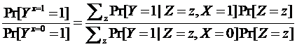
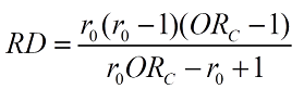
The causal risk ratio for X can be computed by standardization across strata Z as follows:
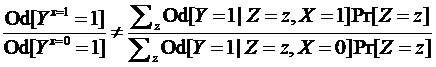
The causal odds ratio for X was considered non-collapsible because it could not be standardized across strata Z as follows which was the classical definition of non-collapsibility:
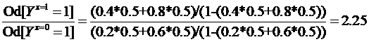
It seems that the causal odds ratio for X should be computed by standardization of probabilities alone across strata Z as follows since odds should emerge from risk standardization:
So does this not mean that odds ratios are collapsible given that the stratum specific ORs are 2.67 while the “risk-standardized” OR is 2.25 consistent with the marginal OR? The scientific question of interest here is whether the question raised about the collapsibility of odds (and thus ORs) is because instead of converting standardized risks to odds we directly attempted to standardize odds. Perhaps this demonstrates that we should always think in terms of risk regardless of the use of odds ratios - they are just a tool to enable us understand risks better.
Edit 1: Third equation edited
Edit 2: Second equation edited
Please edit your post to explain the ultimate goal of the estimand. You seem to be making a number of big-picture assumptions that may not be true. Also check that it is valid to uncondition odds by multiplying by the probability of the conditioning event. I don’t think it is. Such multiplication is used to uncondition probabilities.
You may be right. To be honest I am not too sure myself hence this post but better I take this offline directly with Miguel Hernan as I am referring to standardization as he defines it in his book
Okay, let me give your queries some thought … will edit it and flag the edits at the end of the post. Have to think about your comment on unconditioning odds using probabilities
Edit 1: I gave this some thought and after thinking about this I conclude that standardization is a form of weighted averaging using population weights (as opposed to variance weights which then would make this a meta-analysis and not standardization) so standardizing ORs using probabilities
a) Does not uncondition the odds (agree with you)
b) Does define the collapsibility issue. Miguel says in his book “We say that an effect measure is collapsible when the population effect measure can be expressed as a weighted average of the stratum-specific measures. In follow-up studies the risk ratio and the risk difference are collapsible effect measures, but the odds ratio–or the rarely used odds difference–is not (Greenland 1987).” so this weighted average I have defined above (using probabilities) seems the correct definition of non-collapsibility in this example since its value is on one side of the stratum specific estimates in the absence of confounding.
To uncondition an odds ratio I would have thought that you must uncondition the underlying probabilities then build back the OR from these actual probabilities.
It is not appropriate to speak of population weights unless you have access to population weights, i.e., the sample was a random probability sample from the population and you know the sampling probabilities. Many authors have confused population weights with sample weights from non-random samples, i.e., convenience samples with unknown weights. And if you narrow the focus to what is available, i.e., you uncondition with respect to the covariate distributions in the sample, you have not accomplished very much.
I thought so too - hence the equations in the first post but then if we do so the weighted average risks, when built back, take us to the marginal OR
In terms of weights my understanding is that choice of weights depends on purpose so I just used that term more generally (as an example) to refer to non-variance weights in general. In this case we have weights whose purpose is to equalize the frequency of the “values” in a data set aka standardization. I agree very few papers actually do this for odds as I did above but there is an example. But when one says the stratum specific ORs are the same but the marginal is different then the implication is that there are no sets of weights that can “collapse” the two strata values on to the marginal value.
Thanks, this really helped clear my thoughts. Lets consider that the example above is the same study you presented with X being the treatment indicator, Z being sex and Y the binary outcome of interest. We know that delta_p and delta_logit are approximately linear (see next post) and therefore the conditional OR of 2.67 is computed based on the logit increase induced by a particular risk increase induced by X. The marginal OR is 2.25 so this must mean that the two groups defined by X are closer together in terms of risk based on the distribution of the prognostic sex variable in the sample. Several questions I have tried to raise now become clearer:
a) All the discussion thus far points to the OR being collapsible and indeed a weighted average of risks can be built back to the marginal OR as indicated above. We can only consider it non-collapsible if odds are standardized but the implication of doing so is equal to the second equation above which as you suggested is problematic - so which way do we go?
b) You have said that the interpretation of the marginal OR is that the sample-averaged OR (in this example 2.25) does not apply to males, does not apply to females, and can conceivably only apply to a patient whose sex the physician refuses to know and for which their probability of being female is exactly 0.5. Can we also say that the marginal OR applies to either sex albeit with systematic error induced by lack of sex information? Thus a marginal OR then becomes a less accurate OR but for that reason must “differ” from the conditional OR because of interference by a prognostic third variable so why should we be surprised?.
A disagreement with classic epidemiological thinking also emerges based on this line of reasoning: If we were to agree with points a) and b) above then it follows that multiplicative product terms should not be interpreted as multiplicative effect modification as effect modification should refer back to the natural additive (RD) scale. However the product terms on either the RD or OR scales should be consistent with each other such that effect modification on one scale means effect modification on the other (with minor discrepancy - see next post). Only the product term on the RR scale seems non-interpretable in terms of effect modification (not so RD or OR except that RD is non-transportable),
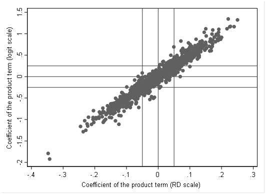
I have been thinking about this some more and realize that a few edits need to be made to my previous post which I will do soon. Just to take this further, I expanded the data in the first post 2500 fold so that there were a million data points. I then created a repeated (1000 times) random sample of 400 from this total population and ran three binomial family GLMs (logit, log and identity links) with inclusion of a product term. The relationship between the logit and identity model product terms is depicted below
On average a 0.01 increment in the coefficient for the product term on the RD scale is associated with a 0.05 increment in the coefficient of the product term on the logit scale thus it is clear that both can be interpreted in terms of additive effect modification and a multiplicative product term (OR scale) is only important in its interpretation in terms of the natural scale. Given that the relationship is not exact there will be inconsistencies especially when the product term is close to zero in which case the margins plot should be able to resolve this since it takes us back to the natural scale. Of interest, this means that if is possible for the effect of X on Y to have the same stratum specific odds ratios yet the stratum variable, Z, can still be an effect modifier (on the natural scale) - but this should be an uncommon occurrence.
Can you step back and better describe the purpose of the exercise and why you need to simulate results and not just write down the math? And please write down the math.
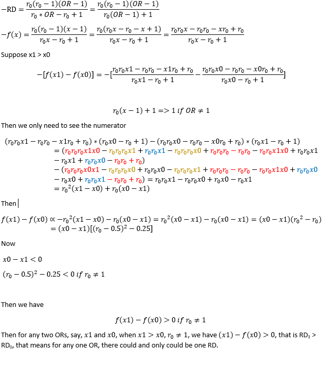
So the simulation results suggest that several pairs of baseline risk (r0) and OR combinations can result in the same RD albeit in a narrow range. Once I work it out will edit this post. Anyone who would like to pitch in - please do
Thanks, I can see that your first step is to indicate that the RD was defined as r0-r1 and you want it to be defined as r1-r0 . I don’t think that matters as the OR would define its interpretation.
If this is a one-to-one function then it means the simulation graph in the previous post is giving us variability due to GLM estimation error? Never imagined it could be that much?
This was because the r0 was considered fixed. If we do not fix r0 then the same fold increase in odds (OR) can have two different RDs.
For example if we have a prognostic third variable Z:
When Z=0 let us assume r0=0.1 and r1=0.5 that is a 9 fold increase in odds but the RD is 0.4.
When Z=1 let us assume the odds of r0 triples thus r0=0.25 and r1=0.75 that is also a 9 fold increase in odds but the RD is 0.5
It is now clear that the simulation variability is indeed because a range of RDs (albeit a small range) map on to the same OR and this (from your proof above) is motivated by variations in baseline risk (r0).
It seems therefore that :
a) Effect modification on the OR scale is a modification of effects by a prognostic third variable (Z in the example above which increases baseline odds 3 fold) but in this example there was no effect modification on the OR scale
b) Effect modification on the RD scale is similar to that on the OR scale except that it is no longer solely about the effect size but rather about impact. The RD of 0.4 and 0.5 are the result of the same “effect size” but have a differential impact as baseline risk changes (in this example an increase in 0.1 over what was observed at baseline risk 0.1)
c) The assumption is that the OR is a measure of effect and the RD is not (akin to the RR).
Edit: A summary of the conclusions from this discussion are posted here as a preprint - please feel free to be as critical as possible if you think the conclusions are not right. Happy if anyone is interested in joining in on it and has any different ideas. Of note, the conclusions have changed quite a bit over the course of the discussion
After giving this more thought, it seems that the most logical conclusion from all this thinking and paying more attention to Frank’s post on statistical thinking is this:
Effect modification should only be considered present when the observed joint effect is inconsistent with the expectation under Bayes’ rule
Since odds ratios are likelihood ratios connecting pre-exposure to post-exposure odds, deviation from the rule means violation of the expected relationship between joint and conditional probabilities = effect (measure) modification.
If so, there is really only one type of effect modification - on the OR scale. The preprint linked in the previous post has been updated for anyone interested to have a look.
An example may bring this into perspective:
Morabia et al published a paper titled Interaction fallacy in 1997. The fallacy was quite simple - the product term on the OR scale suggested that older age at first pregnancy modified the effect of the BRCA1 mutation on breast cancer risk. On the RR scale the product term suggested no effect modification.
If we look at the data reported, without the mutation baseline risk was 6% and with the mutation was 61.5%. Older age at first pregnancy increased risk 1.5 fold at both baseline risks. However the odds increased 1.6 fold at the lower baseline odds and 15.6 fold at the higher baseline odds. They dismissed the latter as fallacious. It is now very clear that the former was fallacious as the RR spuriously declined at the higher baseline risk given that it moves towards the null as baseline risk increases!