Example of situation X: 20 clinical experts are surveyed and the Gini mean difference of their thresholds exceeds 15% so that de facto the threshold doesn’t exist. In general I’d like to see calibration demonstrated in risk interval [a, b] where a is the 0.05 quantile of experts’ thresholds and b is the 0.95 quantile.
So it sounds like you agree that in the scenario given, miscalibration above 50% would be irrelevant (because we said that everyone would have a threshold of 20% or less). I also agree that often “the” threshold doesn’t exist, there is a range of thresholds. The first part of the argument is that calibration outside this range is irrelevant.
Yes. Full calibration curve is mandatory when thresholds aren’t unanimous.
Sorry, I’m confused. Before you said calibration between 0.05 and 0.95 quantile of thresholds; hear you are saying “full calibration curve”. Am i missing something?
I agree that for certain prognostic cases, a model that is calibrated only within a certain range may be useful. A model for survival in the setting of an aggressive cancer might only need to be calibrated in the range of low probabilities.
For decision making, though, expected utility is a function of the distribution itself, so any estimator of that distribution has to be calibrated everywhere.
In other words, consider a binary treatment T, patient covariates X, outcome Y, and utility U. We have E(U|x)=\sum_{y}\sum_tU(y)p(y|x,t)\pi(t|x). To evaluate estimator E_n(U|x) and find the best decision strategy, \pi_n^*=\arg\max_{\pi} E_n(U|x), I think the estimator p_n(y|x,t) has to be calibrated in (0,1).
I am also trying to think about whether this is still the case when evaluating some other function of utility besides expectation.
1 Like
I’m confused about the notation:
- The utility depends on the interaction between the outcome (y) and the treatment choice (T).
- Does p(y|x,t) stands for the estimator? For validation purpose we have the true outcome (y).
NB is deterministic as far as I understand: You should treat patients with outcome and you should avoid treating patients without the outcome. Other considerations (such as treatment-effect or subjective utilities) are implied by the p.threshold.
Sorry that was not clear. Full curve if experts have not been surveyed, quantiles if they have.
2 Likes
Just thinking about this more - I think it’s more complicated than what I originally posted. Actually, we only need that p_n(y|x,t) is calibrated for all x and t. This does not mean it needs to be calibrated in (0,1).
Consider the example where Y is a binary RV representing 10 year survival in the setting of an aggressive cancer, which is unlikely regardless of X, and T is a treatment that does not change things much (so both p(y|x,T=1) and p(y|x,T=0) are near 0). We will have that actually p(y|x,t) is near zero for all t,x. So one can sort of evaluate expected utility in that neighborhood, which will be maybe p(y|x,t) ranging from (0,0.1), because those are the values it takes for all (t,x).
I think overall in this way it is the nature of the probem, as in the example above, that defines the segment of (0,1) on which the model p_n(y,x,t) needs to be well calibrated to evaluate expected utility (or even where it can be well calibrated—for example, if 10-year survival is very rare, then it’s hard to estimate a model that is well calibrated for probabilities near 1). This range may be the “risk range” referred to above.
Another thing to note, for many decisions, it’s not just the provider who makes the decision—it also depends on patient utility, which depend on patient preferences, which are individual.
1 Like
We have that p_n(y|x,t) is the estimator for p(y|x,t). Utility depends on y which depends on x,t, but sure you can write U(y,x,t) too.
Then, for example, T is treatment, eg medication, X is covariates, eg smoking status, Y is outcome, eg 10-year survival (not in a survival analysis sense, just a binary RV)
1 Like
@VickersBiostats is invited to correct me if I’m wrong, but if I understand correctly the implied assumption is that the validation-data is made of untreated patients.
In other words - you don’t validate counterfactual prediction directly, but p(y|x,T=0) while plugging in the treatment effect through the p.threshold.
It is justifiable from a causal perspective by Causal Bounds:
If y=1|T=0 is observed, assuming monotonicity it might be a Complier or a Never-Taker (i.e Treatment might or might not help).
If y=0|T=0 is observed, assuming monotonicity it must be an Always Taker (i.e treatment is not needed).
I’m not sure if I fully understood:
- By p(y|x,T=0) and p(y|x,T=1) do you mean p(y|x,do(T)) and p(y|x,~do(T)) ?
- Treatment might not change things much and both counterfactual probabilities might be relatively high, as in case of drinking orange juice as a treatment and an agressive cancer as an outcome.
- Treatment might not change things much in terms of outcome-prevention, yet it might be extremely harmful in QALY terms: Imagine Chemotherapy for a sympthom-free patient, on that case extremely low p.threshold is unrealistic.
It all depends on how harmfull the treatment is, if the disease is really rare you don’t have much margin between baseline strategies and prediction-model won’t help much either way:
- for p.threshold < prevalence (almost non-harmful treatment): NB-treat-all will be a little bit above NB-treat-none
- for p.threshold > prevalence: NB-treat-none will be the best strategy regardles of how well you prediction model is.
2 Likes
I am going to answer these questions, but just FYI, I re-read the OP’s question, and I think I would need to expand the framework to deal with their question, and maybe I am talking past others who already responded for this reason, so feel free to skip reading. Overall though, the notation/framework I provided before (not really my own) is very elegant and expressive for these types of problems.
I like your example of orange juice for cancer. To better describe the notation, and my argument (which I had thought aligned with Harrell’s conclusion about a “risk range,” but also allowed for this risk range to be a subset of (0,1)), let’s say the following happens.
We run a RCT (in this way, we can avoid bringing counterfactuals into it—actually, I’m not sure we can ever avoid the RCT when decision-making is involved, but that’s another topic) assigning 50 cancer patients to a morning glass of orange juice and 50 to water (orange-colored). Then T=1 if orange juice and T=0 otherwise. We then wait 10 years and assess 10-year-survival, Y, which will be 1 if the patient is still living and 0 otherwise.
We will then estimate the following: p(Y=1|T=t). This corresponds to the “predictive model.” Suppose we get within our data p_n(Y=1|T=1)=0.05 and p_n(Y=1|T=0)=0.10 (orange juice would actually harm cancer patients, because sugar in general is not so good for people). Say utility is U(Y)=Y; i.e., utility of death is 0 and utility of living is 1. So maximizing expected utility is equivalent to maximizing EY.
Now EY = p(Y=1)=p(Y=1|T=1)p(T=1)+p(Y=1|T=0)p(T=0).
Often, p(T=t) is given a special name, \pi(T=t), because it corresponds to the distribution over actions that we have control over; it is a “policy.”
Now EY = p(Y=1|T=1)\pi(T=1)+p(Y=1|T=0)\pi(T=0) and
(sorry, not sure how to \begin{align} in markdown), E_nY= p_n(Y=1|T=1)\pi(T=1)+p_n(Y=1|T=0)\pi(T=0) =0.05 \pi(T=1)+0.10(1-\pi(T=1))=0.10-0.05\pi(T=1), and the game is to find \pi(T=1)\in [0,1] that maximizes this. In this case, we get \pi(T=1)=0. This policy corresponds to the strategy: don’t assign a morning glass of orange juice to cancer patients.
We only needed p_n(y|t) to be well calibrated in the range (0,0.10) to solve this problem. If it had only been well calibrated in the range (0,0.05), we would have solved it incorrectly, since we needed to plug in an estimate for p(Y=1|T=0)=0.10.
The range we needed it to be calibrated for was innate to the observed patients in the study. In other words, as Harrell mentioned, it is “the data” that defines the range, and within this range, we need good calibration everywhere necessary to evaluate expected utility.
Having written all this, I see actually that the OP’s question is slightly different: the OP asks, when there is diagnostic uncertainty about an MI, then what about the calibration of a diagnostic model for this. This is different from the orange juice scenario in which there was uncertainty about the final outcome and a model for this. The outcome in the orange juice example is in the future, 10-year survival. In the OP’s question, the diagnosis is in the past - the MI either happened or it didn’t. I have not thought too much about this problem actually - it’s a related, but different decision problem. I have read Vicker’s paper on prostate cancer as it relates to this.
My sense is that because still one would have to evaluate expected utility, one would still be constrained to have the diagnostic model be well calibrated within a range that is necessary to do so. This range again will be linked to the population under investigation in the decision problem (ie, the population from which the data will be generated), and this may not be between 0 to 1, depending on how how rare the diagnosis is, for example.
3 Likes
Good thinking. There is an important point that I doin’t think has been covered earlier. The decision with the optimum expected utility is a function of not only risk point estimates but also of uncertainties in estimated risk. The weight of the uncertainties in the calculation is especially important if the uncertainties are asymmetric. For example the posterior distribution of risk may be very asymmetric but one of the tails may not be consequential for the decision. So it’s important to ultimtely do a complete integrated analysis that incorporates the whole posterior distribution of risk.
2 Likes
There’s a slightly different framework for RCTs, you’ll have to use a threshold for the treatment-effect and provide individualized estimates for the risk reduction. That’s different from conventional NB that assumes implicit tretment-effect through the probability-threshold.
Avoiding orange juice might increase your survival probability, would you give up orange juice for 0.000000001% risk reduction?![]()
The ATE you mentioned is just an average for the group.
That’s an extremely important point, even though the algebric mechanism is identical the concept is different: The orange juice example relates to prognosis, and the cognitive obstacle is related to counterfactual thinking implied within the algebra.
We always pay a price for being agnositc, and the diagnostic framework has it’s own:
Do you mean some like this?
3 Likes
Well, you guys have been getting on well without me, while I wrapped up some grants! A few thoughts come to mind:
- For the more common type of decision curve analysis, where the prediction is the risk of the event (e.g. risk you have cancer on biopsy) not the difference in risk of event (e.g. reduction in risk of heart attack if you take statin), you have to do this on a cohort that was all treated or untreated, it can’t be a mix. An example of all treated would be in patients getting biopsied for cancer. A model trying to predict cancer would then be used to identify patients who were at low risk and so didn’t need a biopsy. One interesting point here is that you now the counterfactual, what would have happened had they not been biopsied (e.g. a cancer would have been missed. An example of no-one treated would be patients getting surgery only for cancer treatment. A model to predict recurrence would be used to identify patients who are at high risk of recurrence, and would therefore be referred for adjuvant therapy. In this case, you don’t have the counterfactual (i.e. would the patient have recurred had they gotten adjuvant?) you are thinking about the counterfactual more implicitly (e.g. patients getting adjuvant have a 25% relative risk reduction).
- However you do your notation, it makes no sense that calibration would make any difference to utility if you are far from any decision threshold.
- Frank makes a not unreasonable point, which is that experts have not been consulted, you need to show the full calibration curve. My view is that if you don’t know the thresholds, the model is unusable anyway so the issue of calibration is neither here nor there.
- In several of the discussion points, authors talked about calibration as if: a) it was a binary, models are either well-calibrated or they are not, and b) it is relatively straightforward to judge whether calibration is ok or not. I am skeptical on both of those counts. All models have some degree of miscalibration. To determine whether that degree of miscalibration is problem, you have to look at clinical implications, e.g. assess net benefit and do a decision curve. Or to put it another way, when you say “we need model calibration to be good in the range (y1, y2)”, you mean “we need the model calibration to be good enough in the range (y1, y2)” and how you tell “good enough” is to use a decision analytic method.
- The published version of Bayesian decision curves is here Bayesian Decision Curve Analysis With Bayesdca - PubMed. I actually find this paper highly problematic. First off, they show decision curves with Bayesian uncertainty intervals. These are obviously misleading in the same way as showing two point estimates with 95% CI for treatment vs. control arm in an RCT is misleading (the 95% CI can overlap even for a statistically significant result). It is actually worse than that, because the uncertainty intervals are correlated (e.g. if net benefit to treat all goes up, so does net benefit for treat by model). Second, the paper is not actually decision-analytic. It involves the idea of “risk aversion” vs. “risk neutrality” as if these are easily distinguishable binary natural states and talks about aspects of prediction model implementation, such as infrastructure and training, as “irrecoverable costs”. But of course, not implementing a beneficial model leads to “irrecoverable costs” for the patients who get suboptimal care as a result. The standard decision analytic approach to this sort of problem would be to quantify the harms of model implementation (largely economic) and compare those against the harms of delayed implementation (in terms of poorer patient care)
4 Likes
We’ll have to have a friendly disagreement about that. Medical practice involves a huge amount of individual physician decision-making, and a significant portion of that is risk-based. In addition, the use of thresholds assumes that patients have no say in the matter. So given a trustworthy risk estimate, lots of decisions are made without thresholds, or you could say using dynamic on-the-spot thresholds.
1 Like
How can you make a decision without a threshold (even if it is a bit fuzzy and / or dynamic)?
Do you take prevention into account?
If not, the interpertation of treat-all as a baseline strategy is straightforward:
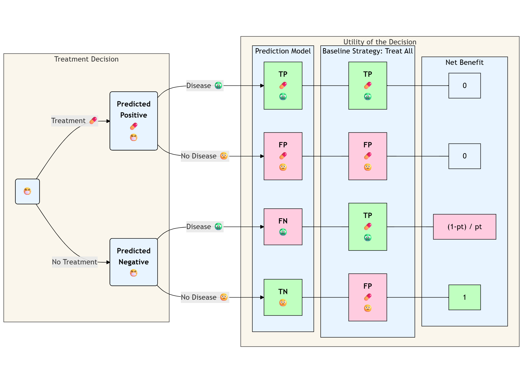
Otherwise it might be misleading to think about observed classifications the same way we are used to. “True-Positive” for treated patients is a bad think in the context of outcome prevention:
The observed utility for y=1,t=1 is 1-event-trt, i.e these patients would be better off without the useless and harmful tretment (counterfactual utility for y=1,t=0 is 1-trt).
1 Like
The traditional method here is to calculate net benefit for treat all and treat by prediction, take the difference and divide that difference by the odds at the threshold. That gives you the reduction in interventions compared to treat all.
1 Like
I know that and it make sense to me if the observed-outcomes are generated from a fully untreated cohort.
But I struggle to understand how it make sense for a fully observed treated cohort:
An individual that has been observed with an outcome and a treatment is better-off without the treatment doesn’t he?
1 Like
I think that 99% of decisions are made without thresholds, by just playing the odds. You might argue that there are internal unspoken thresholds at play in those cases but that has the same effect as not having a threshold. More than 1/2 of medical practice is not even based on data.
1 Like