we are interested in applying the ordinal longitudinal model to model diabetes complications using electronic health data from the Health Protection Agency of Milan but we have some doubts that we would love to discuss with you. The aim of the project is basically to identify patients at higher risk of complications in order to call them for a follow-up visit.
Diabetes complications are captured by contacts with the National health system and might be modelled as a composite time-to-event point.
We wanted to model complications by the ordinal longitudinal model by ordering the gravity of the different events. As the occurrence of events could only worsen the disease stage of the patients, we did not allow backward transitions.This is in line with modeling it as a sort of disease stage, in which stages of disease can only get worse.
The question is whether you have ever applied the ordinal longitudinal model in a situation in which backward transitions are not allowed and if the model is suitable for that or would need some adjustment.
When we tried to apply it in a simplified situation (without covariates) we got a strange result.
The state occupancy probability (SOP) of the baseline stage (no event/no complication) resulted 85%, incoherent with the Kaplan-Meier estimate of event-free survival (using the composite end-point, 63% that is also the percentage of patients who did not experienced any event in the follow-up - here censoring is quite rare). Regarding the absorbing state of mortality, this was estimated to be around 10% in standard SOP, while 820 (22%) deaths were observed in 3684 patients.
We tried to fix it by implementing a costrain of no backward transitions in the SOP (we can provide code), but we think this should be accounted for in the model itself, then we would love to hear your opinion on that.
Please note that for the moment we applied the model on a selected subgroup of patients with diabetes (at particularly high risk of complications) as we had computational difficulties in running the model on the whole cohort of 160000 patients.
At baseline everyone is in State “1.no Event”. Afterwards only forward transitions are observed: “2. Amputation”,“3.CardioCerebroVascular Event”, “4.CKD”,“5.Death” with state 5 absobing.
1 Like
The model should already allow for this, and since the outcomes are assumed to be ordered there is no cost of having the model mathematically allow for backwards transitions that are not used. When you fit the model without covariates do you also ignore time and only use previous state as a covariate? Not only is time almost always important (i.e., transition probabilities are not constant over time) but time often interacts with Y in the sense of there being non-proportional odds in time requiring the use of a partial proportional odds model for the time part of the model. This allows there to be early events of one type and late events for another type.
1 Like
Dear Prof. Harrel, thank for your reply. When you say that the model “should already allow for this” do you mean that we could specify some constraint to enforce/model only forward-transitions or you mean that the model learns that they are not possible estimating negligible/very low probabilities of getting back to previous states? In spite of this, should the SOP computations be reviewed to accomodate this? I apologise if I did not fully understand your answer. Thanks in advance!
1 Like
No constraint should be needed. Parameter estimates for moving back to one of those states should be very small, so the model should learn this. The lack of fit you are seeing is probably due to something else such as the 2 things I mentioned.
2 Likes
Dear Prof. Harrel, as far as the two liely issues you referred to, we originally included time as covariate with the following:
model1<-blrm( propagated_event_ordinale ~ propagated_Prev_event_ordinale + week ,
data = k,
iter = 1000,
chains = 4,
file=‘markov2-bppo.rds’ )
and we got a SOP (imposing as baseline state “noEvent”) equal to ~85%. As soon we included interaction between time (week) and previous state, as:
model2<-blrm( propagated_event_ordinale ~ propagated_Prev_event_ordinale * week ,
data = k,
iter = 1000,
chains = 4,
file=‘markov2-bppo.rds’ )
we obtained analogous SOPs (~86%) for the noEvent state at the ending time of the follow-up.
Both these estimates were different from what we expected: by looking at the Kaplan Meier estimator of the composite event (see previous posts) that resulted in a probability of being free from any event of 63%. Do you have any further possible explanation of these results?
You have once again ignored possible non-proportional odds in time.
Dear Professor Harrel,
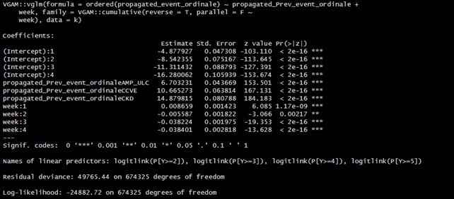
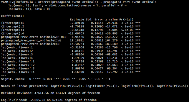
we explored several parameterisations of the model, using the VGAM package. As a first attempt, we allowed time flexibility through splines. Furthermore, we allowed time (both linear (1) and spline-based (2)) to have a partially proportional effect. Comparing the models with different assumptions on the effect of time, we selected the model with PPO of time approximated by splines through the likelihood ratio test.
1)
2)
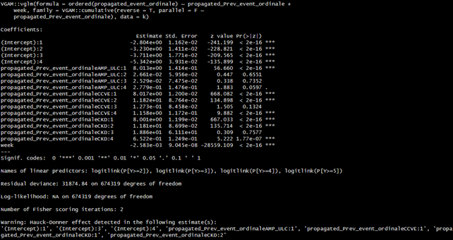
Then we applied a model in which the previous event had a partial proportional effect and a model in which both time (linear and spline-based) and the previous state had a partial proportional effect.
Unfortunately, the models with PPO on previous disease states were not comparable as the likelihood ratio could not be calculated such models returned NA as a result of log-likelihood (3). This is a result that we could not explain: those models warned that the Hauck-Donner effect was identified in some of the intercepts and effect estimates of previous states. Is this a plausible cause for the failure of the log-likelihood calculation?
When we allowed PPO for previous stages, the model, as expected, estimated high probabilities of recurrence on same states or transit to a more severe state, as shown by corresponding estimated parameters (eg propagated_Prev_event_ordinaleAMP_ULC:1, where 1 is the state AMP_ULC). This is in accordance to the dataset structure where we did not allow backward transitions to less severe stages.
Nonetheless we were not able to produce model comparisons in these cases since we could not get log-likelihood values to perform LR tests.
3)
Nevertheless, we were able to produce the SOP graphs. Again, we could not see in the SOP of no events the trend of the Kaplan-Meier estimate calculated on the composite event. In fact, if before (where we assumed PPO for time only) the SOP was ‘too high’ with respect to the KM curve, when previous events had a PPO specification, the SOP of being event-free resulted in a rapidly decreasing path, towards ~ .15. Do you have any suggestions on 1) how to solve the convergence problems (if any) and if they can be due to Hauck-Donner effect, and 2) why we still can’t get the SOP of the event free to mimic the KM on the composite event? Hoping I have made myself clear, thank you sincerely in advance for any suggestions.
It will take me a while to absorb the last paragraph. But to the earlier points I have had trouble getting LR tests from VGAM in similar situations and am fairly certain it’s a bug in VGAM. Try to get the same model using the ordinal package.
Dear Prof. Harrel,
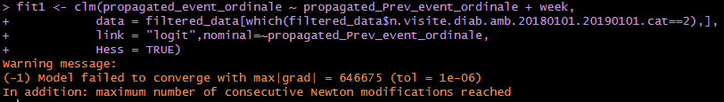
we adopted the ordinal package to perform the test on the same data, but we still encountered convergence problems, so we could not overcome the problem we encountered with VGAM. Here below the code + the warning messsage. In any case, thank you for your valuable comments and support. Either way we will still try to model our settings with rmsb package.
Please remind me of the number of levels of the previous state variable. If it is ordinal and has more than, say, 10 levels you’ll have to treat it as ordinal to limit the number of regression coefficients. For example, you might include a linear and a quadratic term and if the highest level is special in some way also include an indicator variable for it.