The cumulative logistic regression model is commonly applied for ordinal outcomes in the medical literature.
On the other hand, this fascinating article describes the sequential logistic regression model:
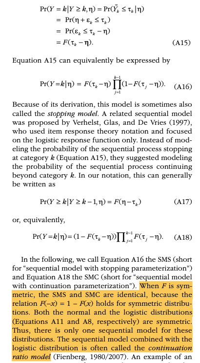
For many ordinal variables, the assumption of a single underlying continuous variable, as in cumulative models, may not be appropriate. If the response can be understood as being the result of a sequential process, such that a higher response category is possible only after all lower categories are achieved, the sequential model proposed by Tutz (1990) is usually appropriate.
Sequential models assume that for every category k there is a latent continuous variable Yk that determines the transition between the kth and the k + 1th category.
I can imagine multiple clinical outcomes suiting these definitions, e.g.:
I didn’t read the paper but my first reaction is the sequential model may be a reinvention of the forward continuation ratio ordinal logistic model, which is a discrete hazard model. A comprehensive case study appears in RMS.
Category-specific effects requires a huge sample size as this is just the polytomous logistic regression model.
The only cohesive way to borrow information across categories is to use a Bayesian prior for the amount of borrowing, e.g., in a partial proportional odds model to specify priors for the departures from proportional odds as discussed in the first link at COVID-19.
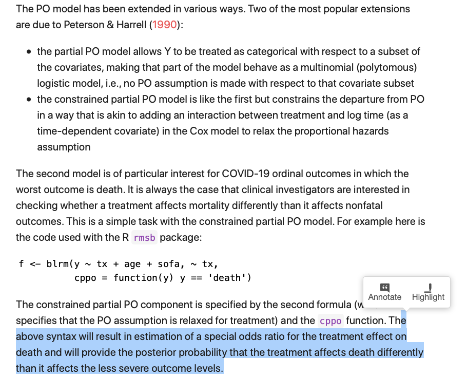
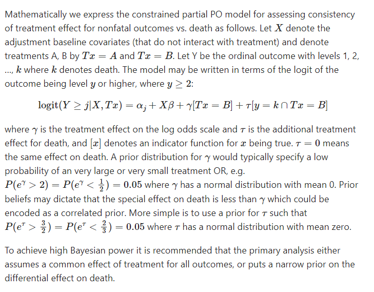
Regarding the text below, please correct me if I misunderstood it: with a constrained partial PO model, one can not only estimate the cumulative OR as in a PO model but also a OR specific to one ordinal score (e.g., death). Would this be analogous to estimate a single category-specific effect?
Would the category-specific effect (CSE) model mentioned in my first post be analogous to an unconstrained PPO model but without shrinkage between CSEs?
Maybe. The clearer situation is that an unconstrained partial proportional odds model that allows non-PO for all predictors is equivalent to a polytomous logistic model.
From my quick experience with the Bayesian PPO model, the SD for the PPO term really determines the amount of shrinkage (e.g., SD = 5 vs. SD = 1). Can I find guidance on how to pick the exact SD value anywhere? This vignette is fascinating but doesn’t discuss this degree of detail.
I wonder if a prior predictive check approach would help in this case. rmsb::blrm() doesn’t seem to support prior predictive check, though. Please correct me if I’m mistaken.
Right it doesn’t support that directly. And yes we need some work that helps us select the amount of skepticism in the departures from PO. It’s not a very difficult problem except to put it into a clinical context. It’s easy if you stick with restrictions on ratios of odds ratios.
I would like to confirm if I understood correctly the following quote in your great material about the degree of skepticism in the departures from PO in a constrained partial PO model:
I understand that the \tau parameter follows a normal distribution with mean = 0, which seems to be the fixed default value in rmsb::blrm(). In the linear scale, this parameter can be interpreted as a ratio of odds ratios with mean = 1.0.
You mentioned above that, in the linear scale, a reasonable prior for \tau could have 5\% of probability density above \frac{3}{2} (or below \frac{2}{3}).
One needs to specify such prior in the log scale. Given a fixed mean value of 0, would the SD of this distribution = 0.246? Hence, the argument “priorsdppo” in rmsb::blrm() would be = 0.246, representing a Normal(0, 0.246^2) prior for \tau?
normsolve <- function (myvalue, myprob = 0.025, mu=0, convert2 =c("none", "log", "logodds")){
  # source: https://hbiostat.org/R/rmsb/rmsbGraphics.html

  ## modified bbr's normsolve()
  ## normsolve() solves for SD (of a normal distribution) such that the tail (area) probability beyond myvalue is myprob
  ## myprob = tail area probability
  ## convert2() converts mu and myvalue to the scale of the normal distribution
  ## If mu and myvalue are OR values, use "log" to convert them to log(OR)
  ## If mu and myvalue are prob values, use "logodds" to convert them to log(odds)

  if (missing(convert2)) {convert2 <-  "none"}
  if (convert2=="log" & mu==0) {
    cat ("Note: mu cannot be 0 so setting an arbitrary value of 1.0")
    mu = 1
  }
  mysd <- switch(convert2,
                 "none" = (myvalue-mu)/qnorm(1-myprob),
                 "log" =  (log(myvalue)- log(mu))/qnorm(1-myprob),
                 "logodds" = (qlogis(myvalue)- qlogis(mu))/qnorm(1-myprob)   )
  return(mysd)
}


normsolve(mu = 1,
          myvalue = 3/2,
          myprob  = 0.05,
          convert2 = "log")
#> [1] 0.2465053