Lohmann, Groenwold, and van Smeden have just published the kind of paper I have been waiting for a long time: Comparison of likelihood penalization and variance decomposition approaches for clinical prediction models: A simulation study. Comparative studies of commonly used model-building strategies in binary logistic regression are extremely valuable, and this research sets great examples with regard to choice of analytical approaches, researcher-unbiasedness of assessments of predictive performance, variety of data configurations examined, meta-simulation analysis, reproducible research, and open access.
In terms of the performance measures evaluated in the paper I give the most emphasis to the root mean squared estimation error, which is the square root of the average (over observations) squared difference between predicted and true probabilities. I do not believe that the c-index should have been emphasized because it is not very sensitive for comparing models despite its usefulness for quantifying pure predictive discrimination for a single model.
I have long believed that data reduction (unsupervised learning) approaches such as incomplete principal components analysis (PCA) are good defaults because of their wide applicability over all types of outcome variables and because they work well with longitudinal data also. PCA has major advantages over lasso and elastic net in not misleading analysts about the ability to stably select predictors especially when colllinearities are present. So the paper is worrying me a bit about reliance on data reduction methods.
If someone asked me what is the leading data reduction technique to include in a simulation study it would be sparse PCA because it essentially does variable clustering while doing PCA, using a lasso penalty to make the PCs sparse and more interpretable, and better handling collinearities. Would the authors consider running more simulations to study the performance of sparse PCA?
The paper mentions several PCA strategies but only two were included in the paper. I would have emphasized the strategy that tries to apply a cutoff for variance explained and includes the first k components in a standard maximum likelihood estimation step. How did performance of the reported PCA strategies differ from the ones not reported?
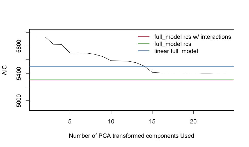
One of the two PCA strategies reported was based on the use of AIC to select the number of components. Did the selection properly force the components to be used in order of decreasing variance explained?
I’m not clear why relaxed lasso was mentioned because it does not have face validity with regard to calibration-in-the-small since the carefully controlled shrinkage in the initial ordinary lasso feature selection step is not inherited by the second estimation step.
Data reduction and shrinkage are most necessary when the number of candidate predictors is large in relationship to the effective sample size 3np(1-p) where p is the proportion of Y=1 (see this). Can the authors provide a graph depicting the root mean squared estimation error (computed against the true probabilities) where something like effective sample size divided by the number of candidate features is on the x-axis?
![]() Related to using AIC to select the first k PCs it would be interesting to see how it works to select k with regard to the effective sample size.
Related to using AIC to select the first k PCs it would be interesting to see how it works to select k with regard to the effective sample size.
Thanks for much to the authors for writing a truly great paper and for considering these requests to provide supplemental information.