I was hoping someone might be able to offer some advice on placing knots for restricted cubic splines. In brief, I am helping a team of clinicians who want to predict which patients require a specialist team to meet them when they arrive (via ambulance) at the hospital. The outcome is severe trauma or not (assessed post-treatment but based on patient condition on arrival; it is a binary outcome) and independent variables are measures the paramedics take at the scene - blood pressure, pulse, etc… It is clear based on contextual knowledge that a non-linear relationship with the outcome is expected; e.g., extremely low or high blood pressure would be associated with worse outcome. As a result, I am using restricted cubic splines; however, I have noticed that for some of the independent variables, there is a small group of patients (approx. 20-30 out of 3000) who score very differently (and not always the same people) and may be exerting large influence on the splines. For example, for oxygen saturation (O2 sats), most people score 80% or above, but there is a group who score in the region 30-70. The expectation would be that as O2 sats increase, probability of severe trauma would reduce. This is indeed what the model returns if I ignore those with O2 sats less than 80 (which I’d prefer not to do) - there is a reasonably rapid decrease in probability as O2 sats increase to ~90% before slowing down - but including them means the probability of severe trauma flattens out (possibly slightly decreases) from below ~90% O2 sats. Is there a better approach than simply trying other knot positions (e.g., moving the first knot to 70-80% or adding another knot around this point) and reporting this is what was done based on the rationale above? I.e., is it justifiable to allow contextual knowledge and some exploration to dictate the approach?
I will here refer to @f2harrell 's beloved Regression Modeling Strategies textbook.
He recommends placing the knots at quantiles, as follows:

Frank also recommends using Akaike’s information criterion (AIC) to help choosing the number of knots (k).
As you have noticed, splines are still sensitive to data scarcity. In my experience, increasing the number of knots - rather than the placements – tend to improve the fit.
I’m currently working on a Shiny app that allows you to toy with non-linearity (of the relationship with Y) and the number of knots. It might help you visualize the impact of k a little better? Feedback appreciated! 
Restricted cubic splines often require pre-specification of knots, and the important issue issue is the choice of the number of knots: the most used number of knots >> 5 knots (=4 df), 4 knots (=3 df), and 3 knots (=2 df).
Pre-specification of the location of knots is not easy, but fortunately location of not is not crucial in model fitting. The number of knots are more important than location! So, practically we may pre-specify the number of knots as " When the sample size is large (e.g., n ≥ 100 with a continuous uncensored response variable), k = 5 is a good choice. Small samples (< 30, say) may require the use of k = 3.
Five knots are sufficient to capture many non-linear patterns, it may not be wise to include 5 knots for each continuous predictor in a multivariable model. Too much flexibility would lead to overfitting. One strategy is to define a priori how much flexibility will be allowed for each predictor, i.e. how many df will be spent. In smaller data sets, we may for example choose to use only linear terms or splines with 3 knots (2 df), especially if no strong prior information suggests that a nonlinear function is necessary. Alternatively, we might examine different RCS.
Ref: Harrell RMS book and Steyerberg CPM book
Excellent answers. A few other thoughts:
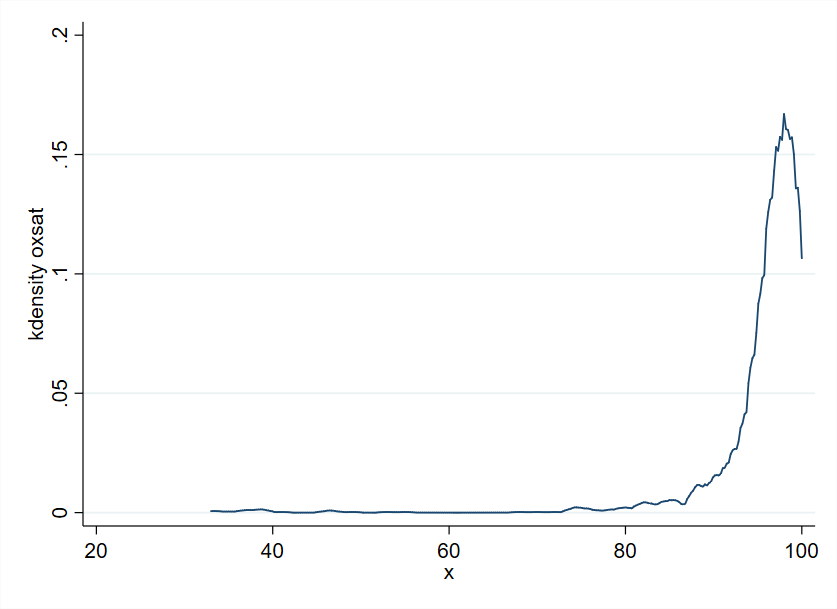
- Include a graph showing the fits with confidence bands, and spike histograms along the x-axis to show the data density for O_2.
- Aside from the fact that the number of knots is the most important aspect of restricted cubic spline modeling, we tend to put knots where we can afford to put knots. Hence the use of quantiles for default knot locations. The spike histogram mentioned above will help on this count.
- Most analysts would just force linearity on the predictor, so you’re way ahead of the game.
Thank you all for your input! It’s greatly appreciated.
I should have given a little more information on what I had attempted so far. I originally planned to use 5 knots based on the locations given in Frank’s book; this results in knots at 88, 95, 97, 99 and 100, though 100 is the maximum score and so was not included - hence 4 knots. I had also looked at using existing clinical thresholds for placing the knots (92, 94, 96). Whilst this latter approach is not sufficient to capture what’s happening in the upper end of the data (as per the default knot placings, 50% of the data is 95+), it has more expected behaviour in terms of what happens below the last knot: the prob of outcome decreases as O2 sats increase, unlike with the default knots. It seems the placing of the last knot is vital - with the first knot below about 89 the line is increasing, and with the first knot above 89 it is decreasing. I think this is a feature of this slightly strange data where 95% of the people occupy 12% of the scale and the remaining 5% are spread across much of the other 88%.
The point re confidence bands is key - the bands are very wide when O2 is below approx. 80 and the changing gradient of the line below the last knot (depending on where it is placed) is a reflection of this. I could be over-thinking it! I believe I should stick with the default knot locations and accept the counter-intuitive findings are a result of uncertainty (reflected in the confidence bands) rather than fudge it so the line looks more like what we expect (and then possibly lend an air of unfounded certainty).
My hunch, if your effect sample size is fairly large, is to put knots at 82 88 95 97 but the suggested graphs would help in the decision.
It would help to see some of your graphs and how knot placement influence the curves.
The first plot is using the default knots (I used 5 knots, but two knots are the same based on the default locations, so only 4 are actually used):

The second plot uses the current clinical thresholds (3 knots):
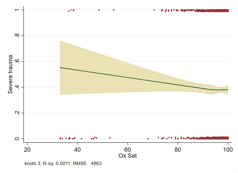
This demonstrates something more like we’d expect for O2 sats below 90 (only in the sense that prob of outcome decreases - whether it decreases at a realistic rate is another matter), though clearly misses something the default knots approach picks up closer to 100.
Thank you for sharing the figures. In my opinion difficult to make much of the “squiggle” you observe when you use 5 knots.
Even with perfectly normally distributed predictors, using many knots can lead to this phenomenon (7 knots in this example):

Same data with 3 knots:
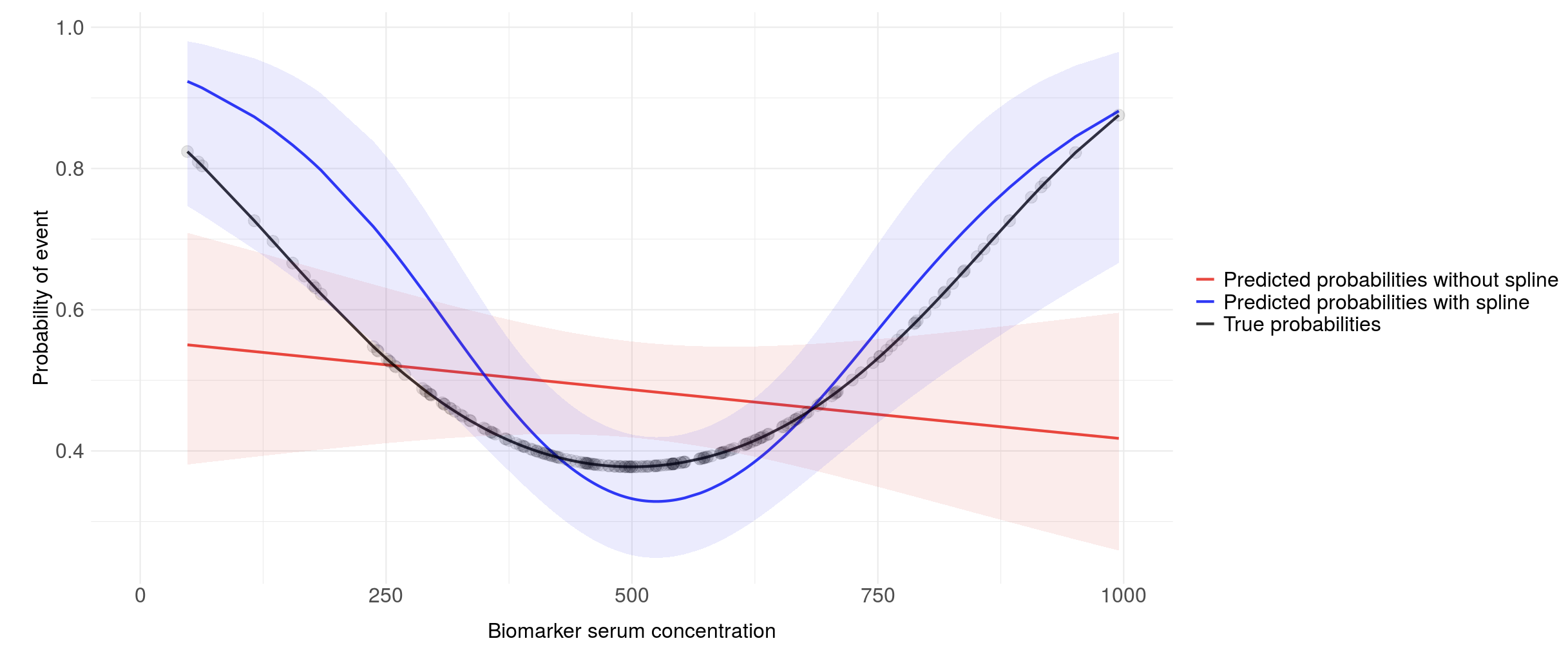
Overall it might still lead to a model that is well fitted and yield better predictions than without the splines.
Given the terribly skewed nature of the data, I’m wondering if data transformation (log?) might be useful here? @f2harrell
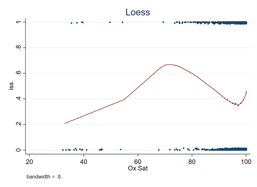
Very interesting. You have strong evidence for non-monotonicity with a nadir at about an O2 of 0.97. I’d be interested in seeing a loess fit, and AIC values for the various knot choices. Having worse results for an O2 sat near 100% smells of measurement error in that part of the scale, or sicker patients getting external O2 support to prop up the O2 sat.
I’ve encountered this before. Setting knots for splines is difficult. If the sample size is reasonably small (not over <2,000 but depends on the model), I’d recommend Gaussian Processes. It’s a great way to fit a non-linear function that requires interpretatability. I’ve had success with this with clinicians in the past. Specifically, in cardiology estimating a non-linear risk function where non-linear relationship is Blood Pressure. The relationship between BP and death is obviously non-linear, we know this from clinical experience.
The best software for this so far is either GPstuff, or GPy.
I’d recommend a logistic linear model:
logit^{-1}(\frac{exp(x)}{1 - exp(x)}) = \beta_0 + x_1 \beta_1 + x_2 \beta_2 + ... + \epsilon
where \epsilon \sim N(0, 1),
for which you specify a non linear prior on each parameter where you expect a non-linear relationship. So -
\beta_{non-linear} \sim GP((x,x') | \theta)
Where for smoothness we select a Radial basis function (synonymous with Exponential Quadratic or Gaussian kernel).
A relevant paper is: Gaussian Process Based Approaches for Survival Analysis Alan Saul.
For many applications GP’s are not applicable, but for this application it works well.
If you’re having issues implementing it, feel free to shoot me an email: andrezapico@gmail.com and I can code it up quickly.
Do you have information on clinical diagnoses of these people ? Either pre-existing or due to whatever brought them into hospital?
There are conditions that would mean their O2 sats don’t follow the same patterns as the average person. COPD would be one common example - folks with COPD typically have much lower 02 sats than the average person of same gender/age.
My limited experience with Gaussian processes is that they fit no better than splines and take much, much more computation time. For this particular application I’d compare with nonparametric regression a la loess.
There is some information on the cause of needing admission (it’s fairly crudely divided into 6 categories: fall from less than 2m, more than 2m, vehicle collision, etc.) but nothing on their clinical history.
Ah right no worries - I thought it worth checking.
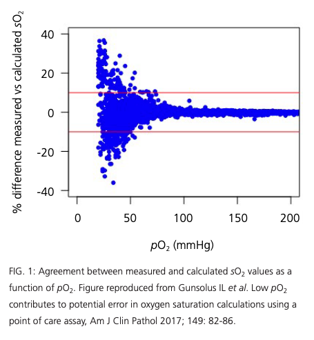
My concern is that you are facing significant measurement errors for lower values of SO2…At the lower end of the tail you have both very few subjects and likely very large measurement errors. A more reliable measurement would be the O2 arterial partial pressure (pO2), unfortunately hard to assess on site.
This is a situation where (I imagine) where you’re likely to have:
- a number of numeric predictors with potentially dramatic effects at either end when you get out of the “normal range” (in the sense of a lab result being “normal”),
- lots of holes in the data, and
- potentially interactions every-which-way.
I’d want to run the data through a Random Forest model, just to see what a totally flexible model that has no moral scruples, and is robust to missing data, would do.
Might not be what you’d go with ultimately, but it’d be a good starting benchmark IMO.
Is this intended to replace triage-by-phone/trauma-team-activation for incoming patients? That’d be a usage case where the validity testing would presumably have to be rigorous^2.