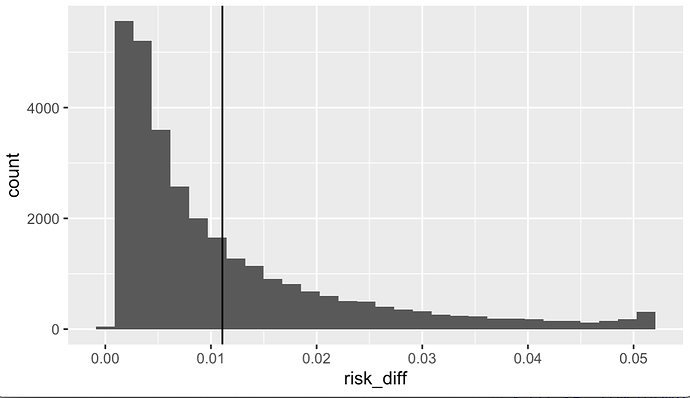
I have been working on a study where the mosts intuitive effect measure would be a risk difference (RD). I am aware that RD has transportability issues, but I am unsure of the significance of this if the study population is the population I intend for the results to apply. My approach is illustrated using the gusto dataset in the Hmisc package. The following code mostly emulates what Dr. Harrell posted here
library(rms)
gusto <- subset(gusto, tx %in% c("tPA", "SK"))

fit <-  lrm(formula = day30 ~ tx + rcs(age, 4) + Killip + pmin(sysbp,
     120) + lsp(pulse, 50) + pmi + miloc + sex, data = gusto)

gusto0 <- gusto
gusto0[, "tx"] <- "tPA"
risk0 <- plogis(predict(fit, gusto0))

gusto1 <- gusto
gusto1[, "tx"] <- "SK"
risk1 <- plogis(predict(fit, gusto1))

df_rd <- data.frame(
  risk_0 = risk0,
  risk_1 = risk1,
  risk_diff = risk1 - risk0
)

ggplot(data = df_rd, aes(x = risk_diff)) +
  geom_histogram() +
  geom_vline(xintercept = mean(df_rd$risk_diff))
Above we have the distribution of individual predicted risk differences, given the model. In the following code I calculated the population mean risk difference and bootstrap confidence intervals.
boot_rd <- function(df){

  df_boot <- sample_n(df, size = nrow(df), replace = TRUE)

  fit_boot <- lrm(
    formula = day30 ~ tx + rcs(age, 4) + Killip + pmin(sysbp, 120) +
      lsp(pulse, 50) + pmi + miloc + sex,
    data = df_boot
  )

  gusto0 <- df_boot
  gusto0[, "tx"] <- "tPA"
  risk0 <- plogis(predict(fit_boot, gusto0))

  gusto1 <- df_boot
  gusto1[, "tx"] <- "SK"
  risk1 <- plogis(predict(fit_boot, gusto1))

  risk_diff = risk1 - risk0

  rd = mean(risk_diff)

  return(rd)
}

rd <- NA
for(i in 1:100){
  rd[i] <- boot_rd(df = gusto)
}

mean(rd)
quantile(rd, probs = c(0.025, 0.975))
Assuming I will show the RD distribution figures and acknowledge that RD may vary considerably with underlying risk, then what, if anything, would be wrong with reporting the population mean RD with bootstrapped confidence intervals in the study text? What assumptions are inherently being made when inferring from the population mean RD?
