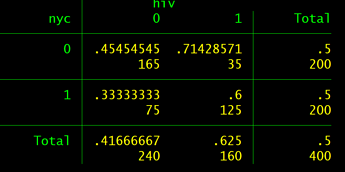
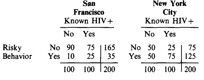
In their paper “Odds Ratios – Current Best Practice and Use”, Norton, Dowd, and Maciejewksi argue that one of the lesser known limitations of the odds ratio from a logistic regression is that it is
…scaled by an arbitrary factor (equal to the square root of the variance of the unexplained part of binary outcome).4 This arbitrary scaling factor changes when more or better explanatory variables are added to the logistic regression model because the added variables explain more of the total variation and reduce the unexplained variance. Therefore, adding more independent explanatory variables to the model will increase the odds ratio of the variable of interest (eg, treatment) due to dividing by a smaller scaling factor.
The implication being
Different odds ratios from the same study cannot be compared when the statistical models that result in odds ratio estimates have different explanatory variables because each model has a different arbitrary scaling factor.4-6 Nor can the magnitude of the odds ratio from one study be compared with the magnitude of the odds ratio from another study, because different samples and different model specifications will have different arbitrary scaling factors. A further implication is that the magnitudes of odds ratios of a given association in multiple studies cannot be synthesized in a meta-analysis.4
(Reference 4 listed as #2 below.)
I was surprised by this given that I am taught to treat ORs as transportable. Inspired by all you fine folks, I looked for an example of a simple simulated logistic regression to check for myself.
In R
 set.seed(666)
 sims = 100
 out <- data.frame(treat_1 = rep(NA, sims),
                   treat_2 = rep(NA, sims),
                   treat_3 = rep(NA, sims))
 n = 1000

 for(i in 1:sims){

 x1 = rbinom(n, 1, 0.5)           # Treatment variable
 x2 = rnorm(n)                       # Arbitrary continuous variable
 x3= rnorm(n)                        # Another arbitrary continuous variable
 z = 1 + 2*x1 + 3*x2 + 4*x3        # linear combination
 pr = 1/(1+exp(-z))         # pass through an inv-logit function
 y = rbinom(n,1,pr)      # bernoulli response variable

   #now feed it to glm:
   df = data.frame(y=y,x1=x1,x2=x2, x3 = x3)
   model1 <- glm(y ~ x1, data = df, family = "binomial")
   model2 <- glm(y ~ x1 + x2, data = df, family = "binomial")
   model3 <- glm(y ~ x1 + x2 + x3, data = df, family = "binomial")


  out$treat_1[i] <- model1$coefficients[[2]]
  out$treat_2[i] <- model2$coefficients[[2]]
  out$treat_3[i] <- model3$coefficients[[2]]
 }

 colMeans(out)
True enough, my column means were
  treat_1   treat_2   treat_3
0.5980825 0.7585841 1.9987460
So without any interaction between variables but all three being prognostic of outcome, I get three different results for my treatment effect.
So from this, my questions are:
- Have I made a mistake or misinterpreation that easily explains these results?
- I have been taught that when trialists provide adjusted odds ratios to use those for meta-analysis, but wouldn’t this imply that I would be extracting different odds ratios depending on the number of variables that were adjusted for?
- Is meta-analysis of observational trials using odds ratios entirely hopeless since, as stated by Norton et al: “different samples and different model specifications will have different arbitrary scaling factors”?
References
- Odds Ratios—Current Best Practice and Use
EC Norton, BE Dowd, ML Maciejewski - JAMA, 2018 - Log odds and the interpretation of logit models
EC Norton, BE Dowd - Health services research, 2018 - Wiley Online Library


