We are developing a prognostic model for cognitive development in very preterm infants using advanced MRI scans. To achieve this, we used three types of MRI information: functional connectivity (FC), structural connectivity (SC), and morphometry. Additionally, we incorporated clinical data to enrich the model. This resulted in high-dimensional data with more than 1,000 features for each subject, making model development challenging. Therefore, we needed to perform data dimension reduction.
We selected non-negative matrix factorization (NMF) for feature extraction because it facilitates the identification of statistically redundant subgraphs, allowing for overlapping and flexible co-occurrence of components. NMF’s non-negative constraints also ease the interpretability of the subgraphs as additive, positively contributing elements. We applied NMF separately to the SC and FC graph measures. Prior to modeling with NMF, the morphometry data (which included some variables with negative values) were logarithmically transformed and subsequently subjected to Min-Max scaling to meet the algorithmic assumptions of NMF.
After applying NMF to the SC, FC, and morphometry data separately, the dimensions were reduced to 31 for SC variables, 29 for FC variables, and 26 for morphometry variables. We then added 6 clinical biomarkers, 1 cMRI injury, and age at scan (a total of 94 variables).
To develop and evaluate the models, we used bootstrap optimism correction validation and kernel-based SVM. For this model, we used the ANOVA kernel. The bootstrap optimism correction evaluation involved the following steps:
- Develop the model M1 using whole data
- Evaluate the performance of M1 using whole data and ascertain the apparent performance (AppPerf).
- Generate a bootstrapped dataset with replacement
- Develop model M2 using bootstrapped dataset (applying the same modeling and predictor selection methods, as in step 1).
- Evaluate M2 using bootstrapped dataset and determine the bootstrap performance (BootPerf).
- Evaluate M2 using whole data and determine the test performance (TestPerf).
- Calculate the optimism (Op) as the difference between the bootstrap performance and test performance: ( Op=BootPerf-TestPerf) .
- Repeat Steps 3 through 7 for nboot times (n=500 ).
Average the estimates of optimism in step 8 and subtract the value from the apparent performance (step 1) to calculate the optimism-corrected performance estimate for all relevant prognostic test properties.
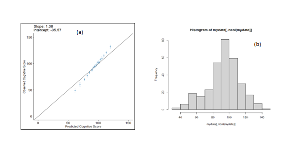
After evaluating the model, we plotted the calibration plot as below, and figured it out, the calibration of our cognitive model is suboptimal while the performance values were high.
If we recalibrated this model, would a new cohort be required to internally validate the model? If so, it may not be worth recalibration this model unless there was a way to do so without losing the ability to internally validate the model. If we recalibrate the model after the apparent performance step but before test performance (i.e., during the bootstrap performance), would the model remain internally valid?
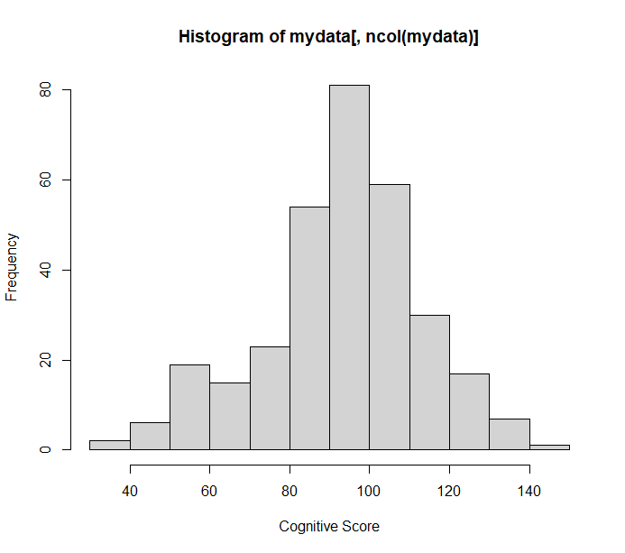
The number of children is 314, and Figure 1 (b) shows the outcome distribution.

Figure 1. (a)Calibration plot of prognostic model for cognitive development, (b) Outcome distribution
Can you provide the number of subjects and a high-resolution histogram of the distribution of Y?
Hi Number of subjects is 314. and this is the high-resolution histogram

With your effective sample size of 314 (since the score is almost continuous) and the dimensionality of potential predictors being extremely high, this type of research is very risky. It would pay off to use your best model to simulate multiple new samples, then to go through all of your analysis steps on the new samples to see if you can reproduce the model used to simulate the data (resimulation, AKA plasmode simulation).
Resimulation typically conditions on the observed predictors so the simulated datasets only replace Y. That means that unsupervised learning will not vary from the original unsupervised learning. That’s not necessary good, but I haven’t thought too much about that.
2 Likes
Dear Dr. Harrel,
Thank you for your response. I was hoping to get some clarification on how to simulate the data. Should I add noise to the existing Y values, or would it be more appropriate to generate new Y values based on the mean and standard deviation?
Thank you for your guidance.
In the Bayesian world this would just be sampling from the posterior predictive distribution. In the traditional frequentist world, re-simulation involves making up or empirically fitting (sometimes using machine learning to allow flexibility but it needs to be interpretable) a model to the whole dataset. Determine the random part of the model and use that to generate new data. For example in a regular linear model, you take the predicted mean for every observation as a population mean and randomly add residuals (perhaps sampling from observed residuals) to generate new Y value. For a probability model such as logistic regression, you take the initial predicted probabilities as true probabilities, and generate new binary data from the Bernoulli distributions corresponding to those probabilities.
I have some R code that may help, once you know what you want to do.
Thanks Dr. Harrel
In our study, we are using kernel-based support vector regression to develop a prognostic model with a continuous outcome. If I understand correctly, I should follow these steps:
- Develop a ksvm model using the entire dataset.
- Evaluate the model on the entire dataset to obtain the predicted values (predicted_y).
- Calculate the residuals using residual = y - predicted_y.
- Generate noise based on the statistical characteristics of the residuals.
- Add the generated noise to the predicted_y to create a new dataset.
- Use the new dataset to develop and evaluate a model, then compare the evaluation metrics of the resimulated model with those of the original model.
If this is correct, my key question is: If we recalibrate this model, would a new cohort be required to internally validate it? If so, recalibration might not be worthwhile unless there’s a way to do so without losing the ability to internally validate the model. Additionally, if we recalibrate the model after the apparent performance step but before test performance (i.e., during the bootstrap performance), would the model remain internally valid?
That sounds good. You may be able to just sample from the estimated residuals rather than having to model their distribution. With the process you outlined, you know the “truth” and can compute the root mean squared prediction error (using predicted minus real condition means). You can also judge stability of found patterns across multiple repetitions of the experiment.
Hi Dr. Harrell
I’ve used the resimulated data to develop and evaluate the model, and the performance was the same as with the original data. Now, I want to proceed with recalibration. My question is: If we recalibrate this model, would a new cohort be required for internal validation? If so, recalibration might not be worthwhile unless there’s a way to do so without losing the ability to internally validate the model. Additionally, if we recalibrate the model after the apparent performance step but before test performance (i.e., during the bootstrap performance), would the model remain internally valid?
This is a difficult issue. @ESteyerberg @Ewout_Steyerberg has thought a lot about this and I hope responds here. I am torn 50-50 on whether a totally new validation would then be required.
Hi Dr. Harrell
Would you please share any references about this method of resimulation?
Also, how can I quantify the level of noise that I added to the outcome by using this residual between predicted and observed outcome?
Thanks
Armin
Hi Dr. Harrell
I also want to apply this simulation to another model with a binomial outcome. How can I do that?
Thanks in advance
Armin

