Hi again professor Harrell, I have rechecked the new feature and I am not sure if it works well or not.
This is the output of redun():
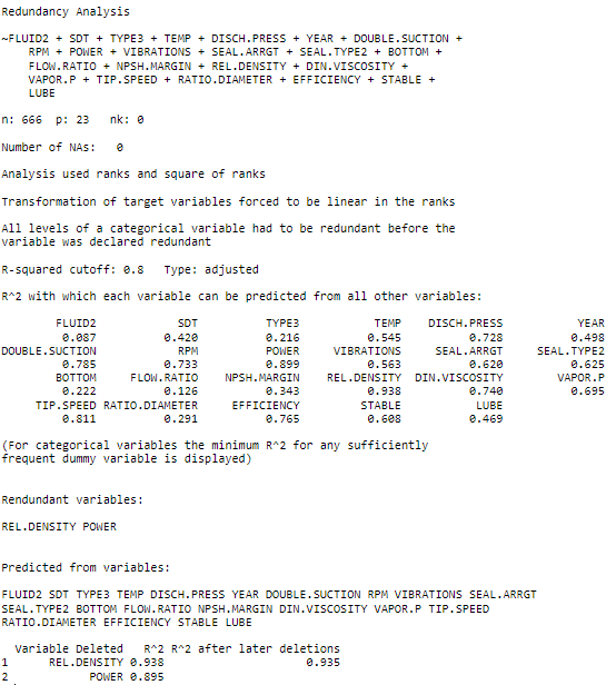
And R2 scores of each variable do not atch with the reduced information given by the output summary of redun() function.
e.g. FLUID2 in the previous summary shows a R2 prediction 0.087 and in the r2$scores a R2=0.892 is shown. Something similar happen to the other covariates.
r2describe(r2$scores)
Strongest Predictors of Each Variable With Cumulative R^2
FLUID2
REL.DENSITY (0.757) + DIN.VISCOSITY (0.861) + VAPOR.P (0.872) + TIP.SPEED (0.879) + YEAR (0.883) +DISCH.PRESS (0.885) + POWER (0.888) +NPSH.MARGIN (0.891) + EFFICIENCY (0.892) + LUBE (0.892)
SDT
LUBE (0.127) + TEMP (0.187) + DISCH.PRESS (0.21) + DIN.VISCOSITY (0.237) + BOTTOM (0.26) + SEAL.ARRGT(0.276) + TYPE3 (0.295) + FLOW.RATIO (0.309) + VIBRATIONS (0.318) + RATIO.DIAMETER (0.322)
TYPE3
DOUBLE.SUCTION (0.667) + POWER (0.732) + TIP.SPEED (0.78) + STABLE (0.801) + LUBE (0.811) + VAPOR.P (0.821)+ RATIO.DIAMETER (0.826) + YEAR (0.829) + SDT (0.831) + TEMP (0.834)
TEMP
BOTTOM (0.086) + POWER (0.133) + VAPOR.P (0.164) + LUBE (0.181) + SDT (0.205) + SEAL.ARRGT (0.219) + TYPE3(0.237) + FLOW.RATIO (0.25) + STABLE (0.253) + SEAL.TYPE2 (0.256)
DISCH.PRESS
TIP.SPEED (0.324) + VAPOR.P (0.373) + LUBE (0.401) + FLUID2 (0.425) + NPSH.MARGIN (0.45) + POWER (0.467) +EFFICIENCY (0.519) + RPM (0.558) + STABLE (0.574) + REL.DENSITY (0.587)
YEAR
VIBRATIONS (0.201) + NPSH.MARGIN (0.285) + SEAL.TYPE2 (0.318) + TIP.SPEED (0.334) + REL.DENSITY (0.363) +SEAL.ARRGT (0.374) + TYPE3 (0.39) + RPM (0.398) + STABLE (0.404) + SDT (0.41)
DOUBLE.SUCTION
TYPE3 (0.667) + TIP.SPEED (0.679) + DISCH.PRESS (0.696) + POWER (0.705) + STABLE (0.709) + RATIO.DIAMETER(0.712) + VIBRATIONS (0.715) + VAPOR.P (0.717) + EFFICIENCY (0.718) + LUBE (0.719)
RPM
TIP.SPEED (0.226) + POWER (0.429) + SEAL.ARRGT (0.508) + DISCH.PRESS (0.546) + STABLE (0.585) + VAPOR.P(0.605) + LUBE (0.618) + TYPE3 (0.626) + EFFICIENCY (0.631) + YEAR (0.635)
POWER
EFFICIENCY (0.472) + TIP.SPEED (0.699) + TYPE3 (0.789) + DISCH.PRESS (0.805) + VAPOR.P (0.826) + VIBRATIONS(0.836) + RPM (0.846) + DOUBLE.SUCTION (0.851) + STABLE (0.855) + REL.DENSITY (0.858)
VIBRATIONS
POWER (0.324) + YEAR (0.424) + TIP.SPEED (0.466) + DISCH.PRESS (0.477) + SDT (0.491) + DOUBLE.SUCTION(0.495) + NPSH.MARGIN (0.499) + LUBE (0.502) + SEAL.ARRGT (0.505) + FLUID2 (0.506)
SEAL.ARRGT
SEAL.TYPE2 (0.269) + RPM (0.398) + NPSH.MARGIN (0.416) +RATIO.DIAMETER (0.436) + TEMP (0.451) + STABLE(0.462) + EFFICIENCY (0.486) + TIP.SPEED (0.5) + SDT (0.511) + LUBE (0.517)
SEAL.TYPE2
SEAL.ARRGT (0.269) + REL.DENSITY (0.382) + EFFICIENCY (0.442) + YEAR (0.455) + NPSH.MARGIN (0.469) + RATIO.DIAMETER (0.479) + STABLE (0.487) + VAPOR.P (0.492) + VIBRATIONS (0.495) + FLOW.RATIO (0.497)
BOTTOM
TEMP (0.086) + NPSH.MARGIN (0.109) + SDT (0.126) + DISCH.PRESS (0.134) + DIN.VISCOSITY (0.143) + REL.DENSITY (0.154) + TIP.SPEED (0.164) + VAPOR.P (0.168) + LUBE (0.171) + EFFICIENCY (0.175)
FLOW.RATIO
VAPOR.P (0.036) + TEMP (0.05) + TYPE3 (0.06) + SDT (0.075) + YEAR (0.081) + DOUBLE.SUCTION (0.084) + POWER(0.087) + STABLE (0.091) + SEAL.ARRGT (0.094) + SEAL.TYPE2 (0.099)
NPSH.MARGIN
VAPOR.P (0.122) + YEAR (0.201) + DISCH.PRESS (0.224) + BOTTOM (0.233) + SEAL.ARRGT (0.241) + SEAL.TYPE2(0.26) + SDT (0.263) + TEMP (0.266) + RATIO.DIAMETER (0.268) + TIP.SPEED (0.27)
REL.DENSITY
FLUID2 (0.757) + DIN.VISCOSITY (0.904) + VAPOR.P (0.921) + YEAR (0.926) + SEAL.TYPE2 (0.927) + NPSH.MARGIN(0.928) + SDT (0.928) + POWER (0.929) + EFFICIENCY (0.93) + DISCH.PRESS (0.932)
DIN.VISCOSITY
VAPOR.P (0.416) + REL.DENSITY (0.473) + FLUID2 (0.643) + TYPE3 (0.668) + SDT (0.679) + YEAR (0.685) + LUBE(0.691) + BOTTOM (0.694) + POWER (0.695) + RATIO.DIAMETER (0.696)
VAPOR.P
REL.DENSITY (0.419) + FLUID2 (0.549) + DISCH.PRESS (0.562) + NPSH.MARGIN (0.577) + DIN.VISCOSITY (0.591) +RPM (0.601) + POWER (0.61) + TEMP (0.618) + TYPE3 (0.624) + STABLE (0.631)
TIP.SPEED
DISCH.PRESS (0.324) + FLUID2 (0.458) + STABLE (0.542) + RPM (0.579) + POWER (0.641) + EFFICIENCY (0.706) +LUBE (0.718) + VIBRATIONS (0.724) + YEAR (0.737) + DOUBLE.SUCTION (0.744)
RATIO.DIAMETER
RPM (0.073) + DISCH.PRESS (0.094) + SEAL.ARRGT (0.12) + TYPE3 (0.133) + DOUBLE.SUCTION (0.139) + POWER(0.145) + STABLE (0.161) + SEAL.TYPE2 (0.168) + EFFICIENCY (0.174) + SDT (0.178)
EFFICIENCY
POWER (0.472) + TIP.SPEED (0.619) + STABLE (0.668) + RPM (0.696) + REL.DENSITY (0.711) + DISCH.PRESS(0.727) + SEAL.ARRGT (0.732) + SEAL.TYPE2 (0.736) + RATIO.DIAMETER (0.739) + SDT (0.741)
STABLE
TIP.SPEED (0.211) + EFFICIENCY (0.328) + RPM (0.446) + SEAL.ARRGT (0.48) + TYPE3 (0.516) + RATIO.DIAMETER(0.529) + YEAR (0.541) + SEAL.TYPE2 (0.548) + DOUBLE.SUCTION (0.552) + POWER (0.556)
LUBE
TYPE3 (0.197) + RPM (0.304) + SDT (0.331) + SEAL.ARRGT (0.346) + VIBRATIONS (0.353) + TEMP (0.358) + FLUID2(0.362) + TIP.SPEED (0.365) + POWER (0.37) + EFFICIENCY (0.375)
What are your thoughts about this issue?
Thank you!
Marc