Hello,
I have been using Probabilistic Index models introduced by Thas et al (2012) as an extension of the Mann-Whitney that accommodates covariates in several analyses. More recently, I have learned about the Cumulative Probability models introduced Liu et al (2016) that is also an extension of the Mann-Whiney test that accommodates covariates. They became interesting to me because CPM can also accommodate random effects and I also learned that there is a relationship between Probabilistic Index (PI) and the common Odds Ratio (cOR) presented in De Neve et al (2019) as follow:
I tried to validate this relationship in R:
library(ordinal)
library(pim)
find_pi <- function(cOR){
aux <- function(cOR){
if (cOR != 1)
out <- cOR*(cOR - log(cOR) - 1)/((cOR - 1)^2)
if (cOR == 1)
out <- 0.5
return(out)
}
aux <- Vectorize(aux)
out <- aux(cOR)
return(out)
}
set.seed(1234)
z_clm <- rep(NA, 100)
z_pim <- rep(NA, 100)
pi_clm <- rep(NA, 100)
pi_pim <- rep(NA, 100)
for (i in 1:100){
y0 <- rnorm(100, 4, 1)
y1 <- rnorm(100, 5, 1)
y <- c(y0, y1)
x <- c(rep(0, length(y0)), rep(1, length(y1)))
dt <- data.frame(y = as.factor(y), x = as.factor(x))
fit <- clm(y ~ x, data = dt)
sm_clm <- summary(fit)
cor_clm <- exp(sm_clm$beta)
pi_clm[i] <- find_pi(cor_clm)
z_clm[i] <- sm_clm$coefficients[nrow(sm_clm$coefficients), 3]
dt <- data.frame(y, x = as.factor(x))
fit <- pim(y ~ x, data = dt)
sm_pim <- summary(fit)
pi_pim[i] <- plogis(sm_pim@coef)
z_pim[i] <- sm_pim@zval
}
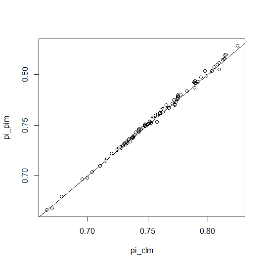
plot(pi_clm, pi_pim)
abline (coef = c (0, 1))
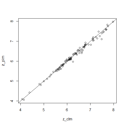
plot(z_clm, z_pim)
abline (coef = c (0, 1))
There are small differences when estimating the probabilistic index. I assumed that the observed differences are numerical. Does that make sense?
However, the differences in Z-score make me a bit more concerned when p-values are borderline.
Then, I tried to re-run a few previous analyses and I found some discrepancies in the conclusions. For example,
library(ordinal)
library(pim)
data('FEVData')
fit_pim <- pim(FEV~ Smoke + Sex + Age + Height, data=FEVData)
sm_pim <- summary(fit_pim)
pi_pim <- plogis(sm_pim@coef)


fit_clm <- clm(as.factor(FEV)~ Smoke + Sex  + Age + Height, data=FEVData)
sm_clm <- summary(fit_clm)
cor_clm <- exp(sm_clm$beta)
pi_clm <- find_pi(cor_clm)

pi_pim
# Smoke       Sex       Age    Height
# 0.3928110 0.5361332 0.5512311 0.5915537
sm_pim
# Estimate Std. Error z value Pr(>|z|)
# Smoke  -0.43551    0.23093  -1.886   0.0593 .
# Sex     0.14479    0.11098   1.305   0.1920
# Age     0.20565    0.02940   6.994 2.68e-12 ***
# Height  0.37039    0.02312  16.018  < 2e-16 ***

pi_clm
# Smoke       Sex       Age    Height
# 0.4193120 0.5513324 0.5432701 0.5895691
sm_clm
# Estimate Std. Error z value Pr(>|z|)
# Smoke  -0.48797    0.26103  -1.869   0.0616 .
# Sex     0.30897    0.14530   2.126   0.0335 *
# Age     0.26021    0.04000   6.505 7.75e-11 ***
# Height  0.54269    0.02735  19.843  < 2e-16 ***
As you can see, there are differences on the conclusion for the variable Sex even though the estimates of PI are very close. What am I missing?
References:
Thas O, Neve JD, Clement L, Ottoy JP. Probabilistic index models. Journal of the Royal Statistical Society Series B: Statistical Methodology. 2012 Sep;74(4):623-71.
Liu Q, Shepherd BE, Li C, Harrell Jr FE. Modeling continuous response variables using ordinal regression. Statistics in medicine. 2017 Nov 30;36(27):4316-35.
De Neve J, Thas O, Gerds TA. Semiparametric linear transformation models: Effect measures, estimators, and applications. Statistics in medicine. 2019 Apr 15;38(8):1484-501.