RMS Binary Logistic Regression

Regression Modeling Strategies: Binary Logistic Regression

This is the tenth of several connected topics organized around chapters in Regression Modeling Strategies. The purposes of these topics are to introduce key concepts in the chapter and to provide a place for questions, answers, and discussion around the chapter’s topics.

Overview | Course Notes

Additional links

RMS10

Q&A From May 2021 Course

  1. Could you please explain how you would come up with a sample size for a logistic regression? I read in your script that one needs 96 participants only for the intercept. Should one then add up 10/20/25 events per variable? FH: We’ll get to that during coverage of that chapter. +1 for this Q

  2. :question: Would you mind summarizing what steps need to be taken to come up with sample size for a logistic regression for an effect? I did not really understand it from what we adressed yesterday…

  3. Can you still adjust for covariates in the scenario where you are predicting two treatments with multiple outcomes? It all depends on the setup of the multiple outcomes.

  4. When should we be worried about large ORs? Can’t think of a problem as long as you accompany them with confidence limits. You’re right, sorry. For example, OR 7.2, 95%CI 1.8 - 28. I want this predictor to be in a logistic model. I just want to understand a good strategy to handle such situations, which are pretty frequent. I’m not sure about the need for a special strategy. Confidence limits document what we know/don’t know and document the difficulty of the task.

  5. Someplace, I think in one of Steyerberg papers, it was suggested to correct the model by “shrinking the coefficients” with bootstrapping, by multiplying them for the bootstrap corrected slope. What do you think about this method of correcting the model for optimism? It is an improvement, but formal panelized MLE is better.

  6. I have the exact same question as the one formulated above. I would like to expand it by asking the following: you have told us that a slope until 0.90 should not worry us much. Nonetheless, if we shrink our coefficients in the model (even if the slope is 0.94 for instance) by multiplying them by the bootstrap corrected slope, aren’t we protecting ourselves even more against overfitting (and that will traduce itself in theoretically better performance in external datasets)? As I see it, the idea of sample size calculation, knowing how many d.f. Are we allowed to spend, performing bootstrap internal validation (optimism correction) and shrinking coefficients all goes in the same direction: to reduce overfitting (or account for it in our final model, as apparent performance will always be too optimistic). Thanks in advance! (pedro). The idea of shrinkage is to shinkage just enough so that there is no overfitting. With severe shrinkage (if you know how much to shrink), you won’t have overfitting, and the effective number of d.f. Is small.

  7. I really liked the simulation with the 5 noise candidate variables in section 8.9 (validating the fitted model) showing what step down selection can do to our slope and R2. Although the example clearly goes against automated variable selection, if we have previously carefully selected our candidate variables based on prior knowledge and literature evidence, theoretically no candidate variable will be noise, right?. Some will have a stronger predictive effect and maybe due to backward stepwise regression we miss a strong predictive variable, but the consequences will not be as dramatic as shown in the simulation, right? I believe the simulation shows us that if matter knowledge is not used previously (for selecting your candidate variables) and you select a bunch of variables that could or could not predict the outcome, then stepwise regression is going to be a big disaster. Also, if the signal to noise ratio is low, then also big disaster? Maybe I am misinterpreting something. Briefly, if you have subject matter knowledge that made you select a variable, it is very unlikely to represent pure noise.

  8. Q for FH & DL: From the statistician’s point of view, the use and understanding of rcs in the logistic regression model is not a problem. However, when used in an observational study (mostly in causal modeling), and when the publication time arrives, results should be presented in a format that can be understood by the editors and reviewers (similar or alternative to uni- and multivariable analysis tables showing ORs and CIs). Plots presenting log-odds/probabilities are OK, but I could not find an ideal way to present findings as a table (also for interactions). I would like to hear your examples or suggestions on this subject. Plots make this very easy. Abandon tables. Another reason the current publishing model has failed us. Interactive graphics with drill-down for tabular details are so much better.

  9. We discussed that the C-index is not sensitive enough to compare two logistic models, is this true also for survival outcomes? If so, what other indexes of model performance do you recommend for survival outcomes? Yes it’s true there too. See Statistically Efficient Ways to Quantify Added Predictive Value of New Measurements | Statistical Thinking

  10. In a case study that a logistic regression was implemented (n= 300, 5 degrees of freedom spent), I found that a risk factor of death or transplant has a large odds ratio equal to 3, however it has a very wide confidence interval (0.73- 14.5). Is it due to a small sample size? Yes

  11. I got this question from a student, and I don’t know the answer. How would Frank or Drew answer? “Is it feasible to compare least-squares regression models to mixed effects models using AIC? I’ve seen some advice indicating it’s okay as long as the mixed effects models use ML instead of restricted (residual) maximum likelihood, as there is no data transformation inherent to the model. Would you concur with this?” I don’t think you can compare them

  12. How can we check which binary outcome rms has assigned a 1 and which a 0? If the outcome is numeric 1,0 already, will this labelling be preserved? It preserves your labeling.

@f2harrell I’m looking for a single “holy grail” performance metric that can be used to compare binary, ordinal, and regression models. Here’s a hopefully realistic scenario that might explain my crazy quest.

In your class, I asked a question about how to properly model financial stock prices. Very often, financial analysts convert the data into a binary “up” or “down” and then try to predict based on various input factors if the stock price goes up or down. You corrected my perspective by explaining that rather than committing the cardinal sin of dichotomizing the continuous stock price data, we should use T1 prices as an input feature (along with any other features of interest) to predict T2 prices. That way, all the the information in the prices is preserved.

So, I want to test if this is truly a superior way to analyze the data. Concretely, I have in mind to reanalyze an article that dichotomized the data and then hopefully show that predicting prices is superior. To do this, I would like to compare three models:

  • Binary: T2_binary_up_or_down ~ T1_X
  • Ordinal: T2_bigRise_smallRise_approxZero_smallDrop_bigDrop ~ T1_X
  • Continuous: T2_price ~ T1_X + T1_price

Essentially, the three models are the same in using the vector of T1_X as input features; the only difference is the amount of information contained in the price (which is stripped of information in the binary and ordinal models). They would all involve the number of rows of data and exactly the same missingness structures.

For a valid comparison, I would like a single performance measure that can evaluate all three models on the same scale. Does such a single measure exist?

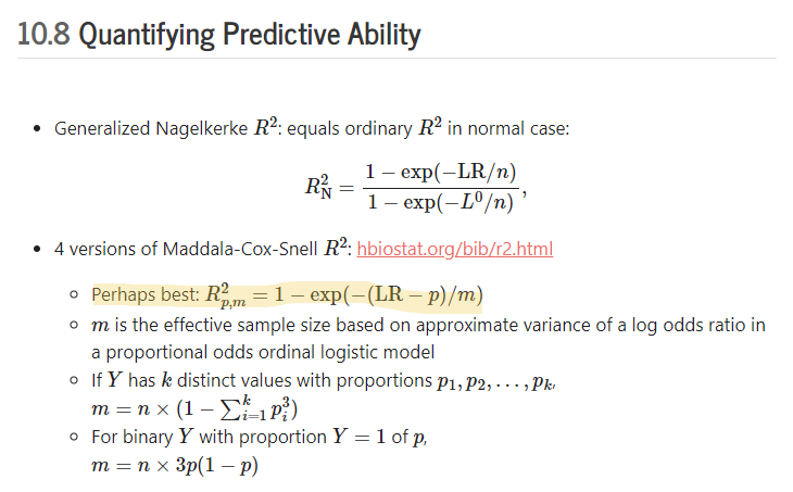
I seem to remember that you recommended the following highlighted R^2 formula:

Is this (or something else) appropriate for my scenario?

I’ve been looking at the Hmisc::R2Measures function, but I can’t seem to figure out how it works; in particular, I don’t understand how to supply the lr argument, especially for continuous models. If something here does the job, could you please help guide me?

At one point I thought that Somers’ D_{xy} rank correlation between predicted and observed was the way to go (simple translation of AUROC for binary Y). But when computed for binary Y it’s bigger than for multi-level Y because predicting a binary outcome is so much easier. Similarly the R^{2}_\text{adj} as you specified is going to make it too easy on coarser Y because it uses the effective sample size instead of the sample size. So for your purpose I would use the traditional R^2 from econometrics (Maddala-McGee etc.) with the actual sample size n used. This will be equivalent to just using the LR \chi^2 statistic for each model. More sensitive models will have larger LR.

Another approach is to consider an effect that is subtle (e.g., some weak but interesting predictor variable, choosing it based only on subject matter knowledge) and show that patterns can be discerned with continuous Y but not with very coarse Y.

I’ll have to get to the R2Measures question later.

Thanks for your response. What exactly do you mean by “the traditional R^2 from econometrics (Maddala-McGee etc.) with the actual sample size n used”? Is there a precise formula for that? Even better, is there an R function for that? Does this work for continuous, ordinal, and binary variables, or is it just for continuous, and then it is equivalent to chi-square for binary?

It’s described in the r2.html page. It’s equal to the last one I listed (my favorite) but reverting back to the apparent sample size.