RMS Describing, Resampling, Validating, and Simplifying the Model

Thank you very much, Dr. @FurlanLeo and Dr. @f2harrell.

I have moved the post here, and if anything I do is inappropriate, please let me know.

First, I want to confirm whether my understanding in the aforementioned post is totally correct, except for the part about the Test sample.

Next, I want to briefly describe my understanding of the Efron-Gong Optimism Bootstrap. (I have the rms book, but for me, I still find many contents difficult to understand, so I would like to get your confirmation to ensure I am not doing anything wrong)

Assuming that there is a model y ∼ k * x, where x is a predictor and k is the coefficient of x, and y is the outcome.

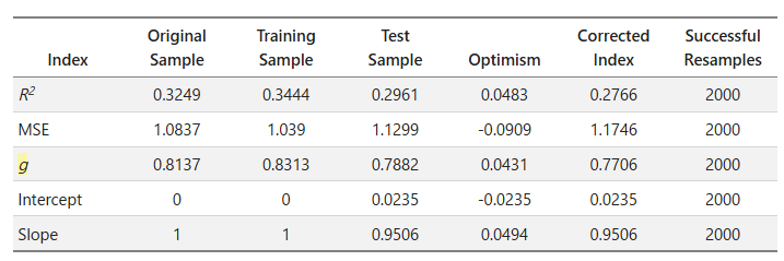
  1. Calculate the performance measures (e.g., R2) in the original data, which corresponds to the performance measures in the Original Sample column in rms.validate.
  2. Calculate the performance measures in a bootstrap sample, and there is a new coefficient k1​ (model: y ∼ k1 * x) in this bootstrap sample.
  3. Use the coefficient k1​ (model: y ∼ k1 * x) to get new performance measures in the original data.
  4. Calculate the optimism by (performance measures in step 2) - (performance measures in step 3).
  5. Repeat steps 2 to 4 for n times to get n performance measures in both bootstrap samples and original samples.
  6. Calculate the average value of the performance measures in step 5, which correspond to the performance measures in the Training Sample (average in step 2) and Test Sample (average in step 3) columns respectively in rms.validate.
  7. Calculate the average value of the optimisms in step 6, which corresponds to the performance measures in the “Optimism” column in rms.validate.
    ie. Training Sample - Test Sample = Optimism

image

Thank you for your patience, and I really appreciate it if anyone could point out any misunderstandings I have. It would be very helpful for me.

2 Likes

I think that’s correct. In Chapter 5 of RMS book and course notes I use different notation that makes it very clear which data are being used, both to fit and to evaluate performance on.

2 Likes

Thank you for your patience and kind confirmation.

Dear all
Thank you very much for this great thread, very instructive. I am trying to develop and validate internally a Cox regression model for a time to event analysis. I have managed to get the bootstrap corrected calibration plot via calibrate function from rms package followed by plot function. Is there a way to retrieve mean calibration from the function? Would the plot be enough by itself?
Thank you very much
Marco

I should have done a better job returning summary stats to the user. Best to look at the code for print.calibrate and print.calibrate.default but first try

cal <- calibrate(...)
p <- print(cal)
str(p)  # see what's there
2 Likes

Hi,
I would like to plot the rank of predictors of a model which is fitted with some restricted cubic splines (using rcs()).

The problem that I face is that each covariate Xi is splitted in all of its components (X,X’,X’‘, X’‘’ and so on) and I would like to plot the rank of each covariate as just one predictor, including implicitly all the exponents.

I use the method shown in section 5.4. of RMS book.

plot(anova(fit), sort='none', pl=FALSE) ...

How can I group all the components of the variable and perform the rank computation?

Thank you so much!
Marc

plot(anova()) does all the grouping automatically.

1 Like

Hi, I’m very sorry for the confusion; indeed, the importance of the variable includes all the factors of the splines.
Thank you professor for the clarification.

1 Like

Dear @f2harrell,

I have a few questions about the validation of an ordinal prediction model, fitted with lrm() and validated with validate() and calibrate, using bootstrap with 500 resamples. I would appreciate if you or anyone else could help.

The sample size for this model is 2,118. The model has 4 intercepts (outcome = 1,2,3,4,5) and 10 degrees of freedom. The model has been internally validated using the third intercept. I have attached to this post 2 figures, one contains the calibration curve with some optimism-corrected performance indexes, and other contains the distribution of the model predictions.

Calibration

Predictions

Question 1
For extracting the 0.9 quantile of absolute prediciton error (0.9qAPE), I did the following:

cal <- calibrate(m, B = 500, kint = 3, group = data$outcome)
p <- plot(cal)
e <- quantile(abs(p), probs = 0.9, na.rm = T)

The argument na.rm = T above is the trick, because p contains 8 missing values (out of 2,118). This means that, for 8 subjects, calibrate() did not compute a prediction error. Do you know why? I assume this is not a problem, since it’s only 8 missing values (out of 2,118). But what if this were to happen again in the future and the number of missing errors are greater? Perhaps this issue is related to the second issue below.

Question 2
When I inspect the calibration object (cal), I see it has 50 rows and 9 columns (because this is the default of calibrate(). The last column is n, which corresponds to the number of bootstrap resamples (500 in this case). However, the first two and the last rows have numbers in n that are smaller than 500 (351, 494, and 434, respectively). Is this a problem? If yes, how can I fix it, since I already included the argument group in calibrate().

Question 3
Related to the above, in the third column of cal, which is calibrated.corrected, the last of the 50 rows has a value greater than 1 (1.009). Is this normal / ok?

Thank you.

This question does not seem related to the topic under which you posted it.

I wish I had time to delve into the details. I think this will require a close reading of the code. I hope you can do that.

Thanks for the incredibly insightful discussions here on validation!

When using 10-fold CV with 100 repeats, performance estimates within each fold aren’t independent of one another but those across repeats are. Is there an appropriate method for calculating confidence intervals for performance estimates that accounts for this?

I can see that this is simple with independent resamples in bootstrap validation, but these simulations lead me to believe that CV may be safest when working with high dimensional data.

Edit: Thank you for the reference Frank, just adding a link to the paper that describes a nested CV method for improved CI estimates.

Computing valid confidence intervals even for a single repeat of 10-fold CV is not easy. Rob Tibshirani has a paper showing how to do that. There’s probably a way to translate his method into getting standard errors/uncertainty limits for averaged repeated CV.

1 Like