Dear all,
I’m developing a prediction model using different strategies (N = 122; DF = 10; continuous discrete response; using lrm()):
- Full model unpenalized;
- Full model penalized (maximization of AIC);
- Full model penalized (penalty yielding effective DF of approx 122/15 = 8);
- Reduced pre-specified model (built using background knowledge);
- Reduced model (built with backwards elimitation of predictors using AIC);
- Reduced model from 5. estimated with shrinkage of coefficients using penalty from either 2. or 3.
I’m validating all these models with bootstrap and also producing calibration measures with bootstrap.
Questions:
Which performance indexes are most usefull/adequate for comparing these models? E.g., Emax, Slope, Mean Absolute Error etc
Which of these models is the most appropriate for making inferences about the relationships between predictor and response?
Thank you
That’s too many models, lowering the chance that AIC can select the best model with reasonable probability. I’d go with subject matter knowledge to the extent possible. Note that AIC is not valid in the stepwise variable selection context. I’d also make sparse principal components part of the game plan.
Good performance metrics into E90 and those described here.
Hi Professor, thank you for the comments/suggestions.
Actually, I was thinking of going with only model 4 in the paper (my firtst choice really). I would fit the other models and show their performance (calibrationwise) just for comparative purposes and to show the audience/readership how models like 1 and 5 are usually not appropriate for the task.
Please note that I’m not comparing these models against each other on the basis of their AIC. I used AIC only to estimate the penalty factor for the full penalized model (model 2) and to perform backwards variable selection (fastbw(fit, rule='p', type='individual', sls=0.157) (model 5). Then I applied the penalty from model 2, or the penalty yielding an effective DF of 8 (model 3), to this reduced selected model*, resulting in model 6.
*as suggested by Steyerberg (page 259 of the 2nd edition of his book, Clinical Prediciton Models):
“For penalized estimates of the regression coefficients after selection, we can
apply the penalty factor that was identified as optimal for the full model, before
selection took place”
By E90 do you mean the 0.9 Quantile of Absolute Error, as reported by calibrate()?
Thank you
1 Like
Yes on the last question. And yes that makes sense if the penalty is estimated for the biggest model.
Thank you Professor. Much appreciated feedback.
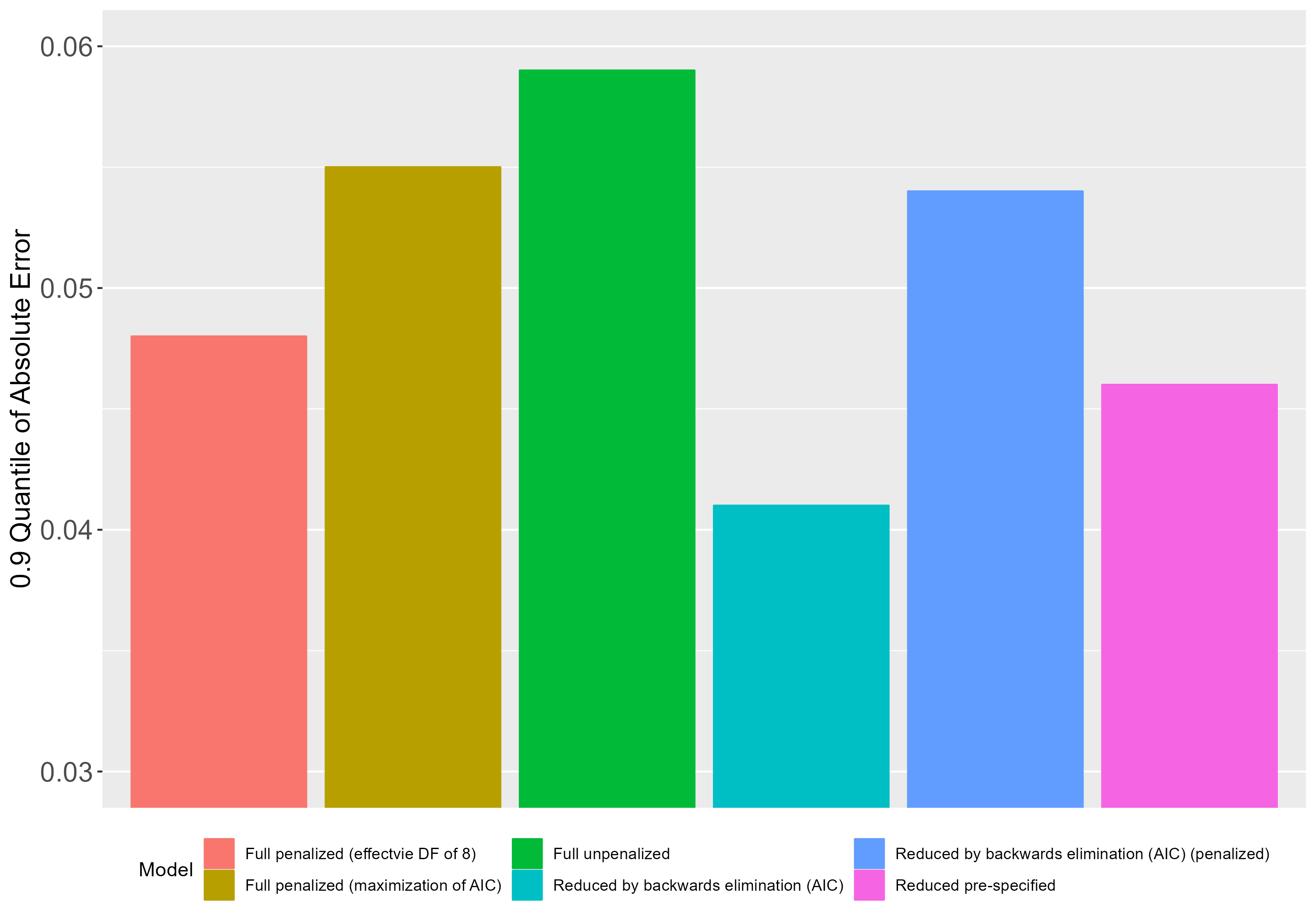
Just to illustrate, here’s a plot with the E90 measures from each of these models.

The model yielding the lowest error is the model selected with fastbw(fit, rule='p', type='individual', sls=0.157 and then validated taking selection into account (4th model from left to right on the plot). This model outperforms the pre-specified reduced model (last model on the plot). Interestingly, if I take the selected 4th model and apply the penalty factor from the full penalized model, this results in worse peformance (5th model on the plot).
Is it safe to perform inference with this 4th (backwards step-down, validated) model?
By inference I mean interpreting partial effects plots and contrasts.
Minor suggestion: horizontal dot charts allow you to more easily read the results because the model labels will be in larger font next to the dots they represent.
I don’t know the answer to your question because
- Calibration, though super important, is only one dimension of accuracy
- You are comparing too many models to be able to avoid damaging model uncertainty
Ok,
Thank you for the great suggestion!
Then I believe that the safest/most appropriate approach here would be not to compare that many models, but simply fit a full penalized model. Perhaps compare (using AIC) 2 or 3 versions of this full model with varying degrees of complexity (in terms of interaction and nonlinear terms) and then select the best one.
The question now becomes: What degree of penalization to use?
The one that maximizes AIC or the one that yields an effective DF of approximately N/15, where N is the sample size. As we can see on the plot above, the latter aproach (which corresponds to less penalization) seems better (at least with regards to the E90 index).
Take a look at chapter 14 of RMS where I use effective AIC to choose a penalty. But beware that there is a sample size requirement to consider for either effective AIC or cross-validation to be reliable for selecting shrinkage parameters.
1 Like
Thank you Professor.
What do you mean by “sample size requirement”?
I have 122 observations and an ordinal discrete response variable, with 36 distinct values. The lrm() model has 10 df with 9 predictors.
When the sample size is small enough to need penalization it’s often too small to be able to guide you in selection of how much shrinkage to apply.
1 Like
Interesting, and rather paradoxical.
I’ve come across this great paper of yours.
- Aren’t you also comparing too many models/strategies here?
I tried to replicate the approach of finding an optimal penalty factor through bootstrap, but couldn’t do it using the rms functions*, so had to do it another way (using a for loop and the dplyr::sample_n function. The problem is that I need to find a way to ensure balanced resampling, so that there is at least one observation for each distinct value of Y in each bootstrap sample (something which is achieved with the argument group when using rms::validate or rms::calibrate).
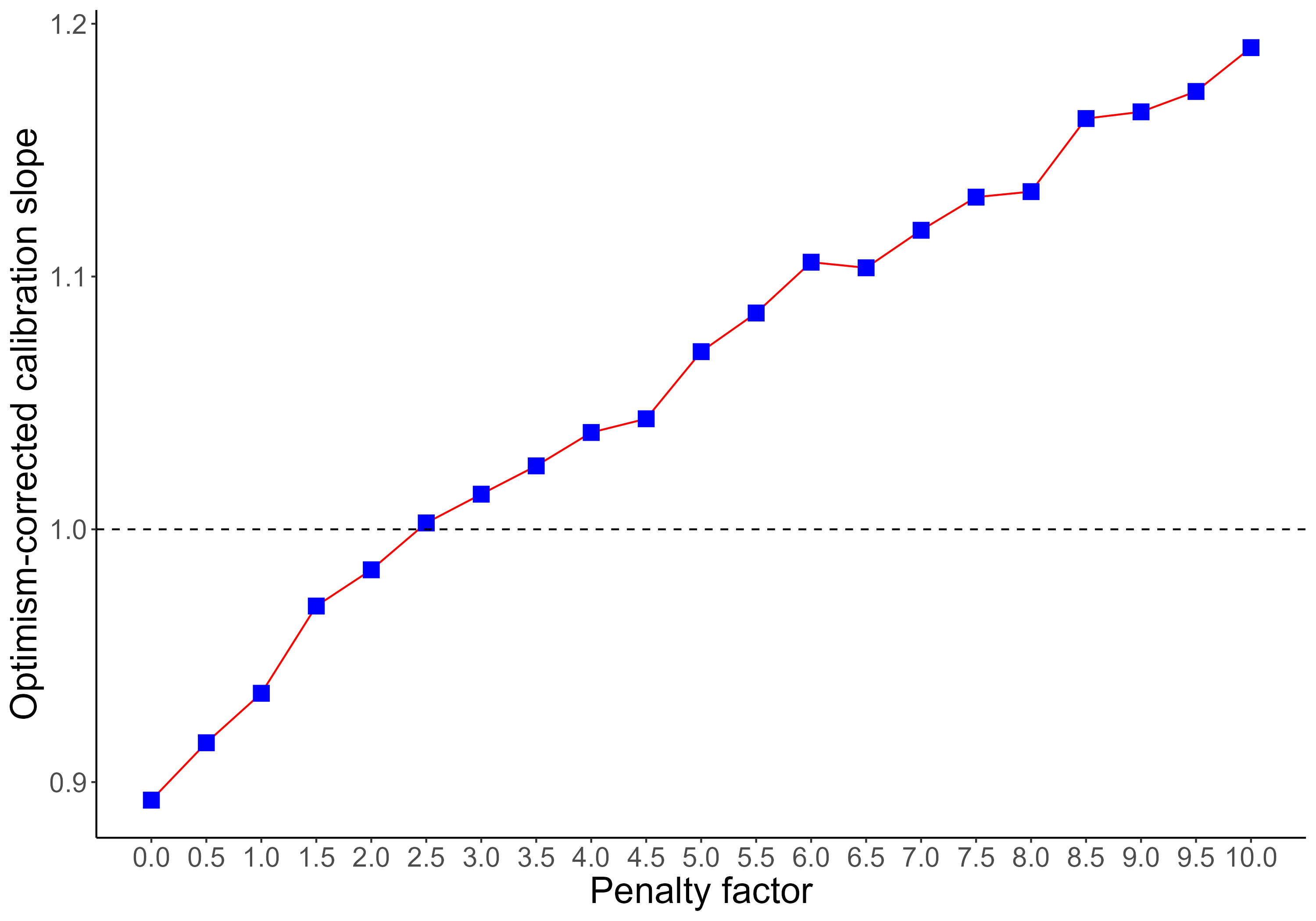
Anyway, I decided to try a different strategy (see plot attached):

To search for an optimum penalty factor by comparing the optimism-corrected (via bootstrap with rms::validate) calibration slope yielded by different penalty factors, and choosing the penalty yielding the calibration slope that was closest to 1.
- Does that make sense?
*I don’t think there is a function to search for the penalty factor using bootstrap, correct?
Thank you again for your attention and invaluable commments.
Hi,
this post comes from this other one that was posted in the wrong place:
https://discourse.datamethods.org/t/validate-and-calibrate-cox-model-on-dataset-with-a-categorical-covariate-with-few-observations/8767?u=marc_vila_forteza
Professor Harrell’s answer:
You may have to combine infrequent levels. Hmisc::combine.levels can help with that. Or use the group= argument to calibrate and validate to do balanced bootstrap sampling. Specify something like group=mydataset$FLUID2 .
→ Thank you for your quick reply. I have another question with regards the use of group=argument. Is it possible to use it for grouping more than one covariate at the same time?
I mean to do something similar to ‘group=c(mydataset$FLUID2,mydataset$TYPE)’.
note: I tested this way to use a vector to specify more than one covariate but it didn’t work.
Thank you
Right there is no built-in function for bootstrapping with penalization-finding.
You can use the interact() function (or is it interaction?) to paste together multiple factors to use in group.
1 Like
Thanks.
What about the strategy illustrated on the plot above? Any thoughts?
It’s useful but would be nice to use a comprehensive measure that rewarded both calibration and discrimination, such as Brier score, mean squared prediction error, mean absolute prediction error.
1 Like
Hi guys,
I am little bit crazy trying to run a penalized cox ph regression model with functions of rms package. I’ve done it with glmnet package but I would like to analize the outputs with rms and Hmisc functions later.
Is it possible to do so with cph() function? as well, how can be performed with cross-validation to found the optimum lambda which leads e.g. to a minimum mean cross-validated error.
Any help or do you have an example to follow?
Thank you
Sorry, no. You’ll need to use the survival package. Start with Section 4.3 of this.
Hi professor Harrell,
I am now checking the cox Lasso regression on my full-original model. After optimizing the value of lambda with a cross-validation procedure, I get a penalized model with its coefficients (I used penalized() package).
fit <- penalized(formula_model, data = g_glmnet, lambda1=optL1fit$lambda, epsilon=1e-5, model = "cox")
After doing that, I tried to run a new model with cph() function, in order to get all the parameters in the format in which I have all the other models and to compare the statistics.
I want to force to have the same model with cph() but I get weird results, as, for example LR X2 = 0.
This is how I am trying to do so:
cph_lasso_fit <- cph(formula_model, data = g_glmnet, init=coefficients(fit,"all"),iter=0, tol=1e-13, x=TRUE,y=TRUE, surv=TRUE, ties = 'efron', id = id)
I understand that I am doing something wrong or maybe it’s not possible what I am trying to do. Can you help me somehow in this issue?
Thank you so much in advance for your help
You can’t feed results of a penalized analysis into an unpenalized fit.
(I copied my post from another thread to here)
Dear professor,
I want to confirm whether my understanding of the columns in the rms validate output is correct.
I know bootstrap can resample. Let me give a simple example. For example, there are 5 values (1 2 3 4 5) in the data set, which is the Original sample. The first resampled sample is (1 1 2 2 4), then this sample is used as Training sample, and then the data composes of unsampled numbers (3 5) is used as Test sample.
The Dxy will be calculated in these three Original, Training, and Test samples as the above, and then n times of bootstrap will be implemented. The standard deviation of n times of Training is optimism.
index.corrected = Original - Optimism (the only special case is Emax in lrm validate)
My understanding of validate is still incomplete. So I hope to get your correction.
(If you are busy and don’t have time to correct me one by one, please tell me where my understanding is wrong, and I will continue to look for information.)
Thank you very much.
Answer from @FurlanLeo :
The Test sample is your entire original sample, not the unsampled values of it.
Answer from @f2harrell :
Yes - this is covered fully in Chapter 5 of the RMS book and in the online course notes. And @JiaqiLi don’t get confused with the “out of bag bootstrap” which is not used in the rms package. We are using the Efron-Gong optimism bootstrap for estimating the bias in an index due to overfitting. This involves subtracting from the original whole sample index the mean optimism. Optimism is from fit in bootstrap sample of size N minus fit index computed from the original sample.
This post is in the wrong place and should have been in datamethods.org/rms5 as instructed at the top of this topic. If. You reply further, copy all that’s been put here related to your question and put it at the bottom of the correct topic.

