RMS Describing, Resampling, Validating, and Simplifying the Model

[Sanne]

Hi,

If a test split is used, can the variability of the performance measure (say RMSE) be assessed by applying bootstrap to the test set? This would be valuable in case smallish test sets are used.

Cheers,

Sanne

[f2harrell]

Think of the bootstrap as telling you how volatile a procedure (e.g., variable selection) is or how imprecise an estimate is (e.g., computing standard errors or confidence limits). The bootstrap doesn’t help with small sample sizes as it inherits the small sample size in all that it calculates. And note that splitting data into training and test requires a huge sample size (sometimes 20,000) in order to not be volatile.

[Sanne]

Thank you! I should have added the goal of the exercise: to show how volatile any performance calculation is on a small test set.

[f2harrell]

The bootstrap will help with that although it may be more direct to simulate multiple small test datasets and show how results disagree across them.

[FurlanLeo]

Please,

Does anyone know how to extract the values of the error measures (Mean absolute error, Mean squared error, 0.9 Quantile of absolute error) displayed on the calibration plot (plot(calibrate(f)))?

I want to insert these values into a data frame for ploting.

Thanks.

[f2harrell]

Start with str(calibrate(...)) to see what’s in the calibrate object.

[FurlanLeo]

Hi Professor, thank you for the suggestion.
I couldn’t find anything related to the errors with str(calibrate()).
But I think I found a way:

c <- calibrate()
p <- plot(c)
mean(abs(p))
quantile(abs(p), probs = 0.9)

The errors are stored in p.

[FurlanLeo]

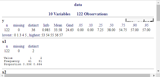
I have been doing some prediction analyses/modeling and could use some feedback.

• The data are displayed on the figure attached, which is a print of describe();
• x1, x2, x3, x4, and x5 are clinical scales/tests usually performed by a physical therapist;
• y is a functional scale (integer values from 0 to 57);
• xs are all performed at baseline and y is measured after ~ 3 months;
• DOM, BAM, SEX, AGE constitute a Base Model:

f1 <- lrm(y ~ DOM + BAM + SEX + rcs(AGE, 3), data = data, x = T, y = T)

• Goal is to determine which of the clinical scales/tests (the xs) add more predicitve power to the Base Model;
• I fitted 6 other Models on top of the Base Model, 1 for each x, with the latter Model featuring a combination of x1 and x2:

f2 <- lrm(y ~ DOM + BAM + SEX + rcs(AGE, 3) + x1, data = data, x = T, y = T)
f3 <- lrm(y ~ DOM + BAM + SEX + rcs(AGE, 3) + x2, data = data, x = T, y = T)
f4 <- lrm(y ~ DOM + BAM + SEX + rcs(AGE, 3) + rcs(x3, 3), data = data, x = T, y = T)
f5 <- lrm(y ~ DOM + BAM + SEX + rcs(AGE, 3) + rcs(x4, 3), data = data, x = T, y = T)
f6 <- lrm(y ~ DOM + BAM + SEX + rcs(AGE, 3) + x5, data = data, x = T, y = T)
f7 <- lrm(y ~ DOM + BAM + SEX + AGE + x1 + x2, data = data, x = T, y = T)

• Then I produced several (optimism-corrected) measures of Model Performance for each Model, using the following code:

validate(f, method = 'boot', B = 500, group = data$y) # internal validation using bootstrap
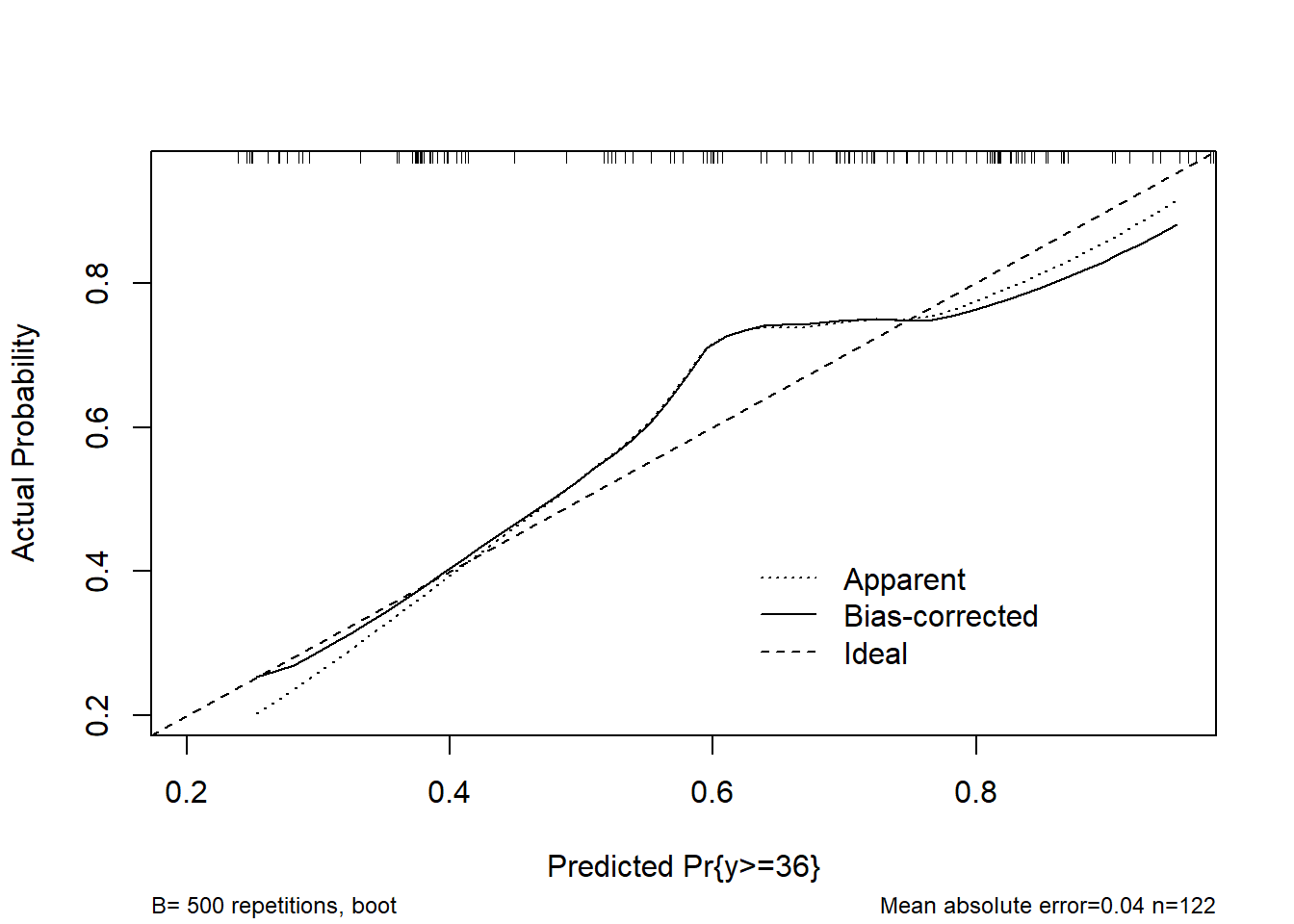
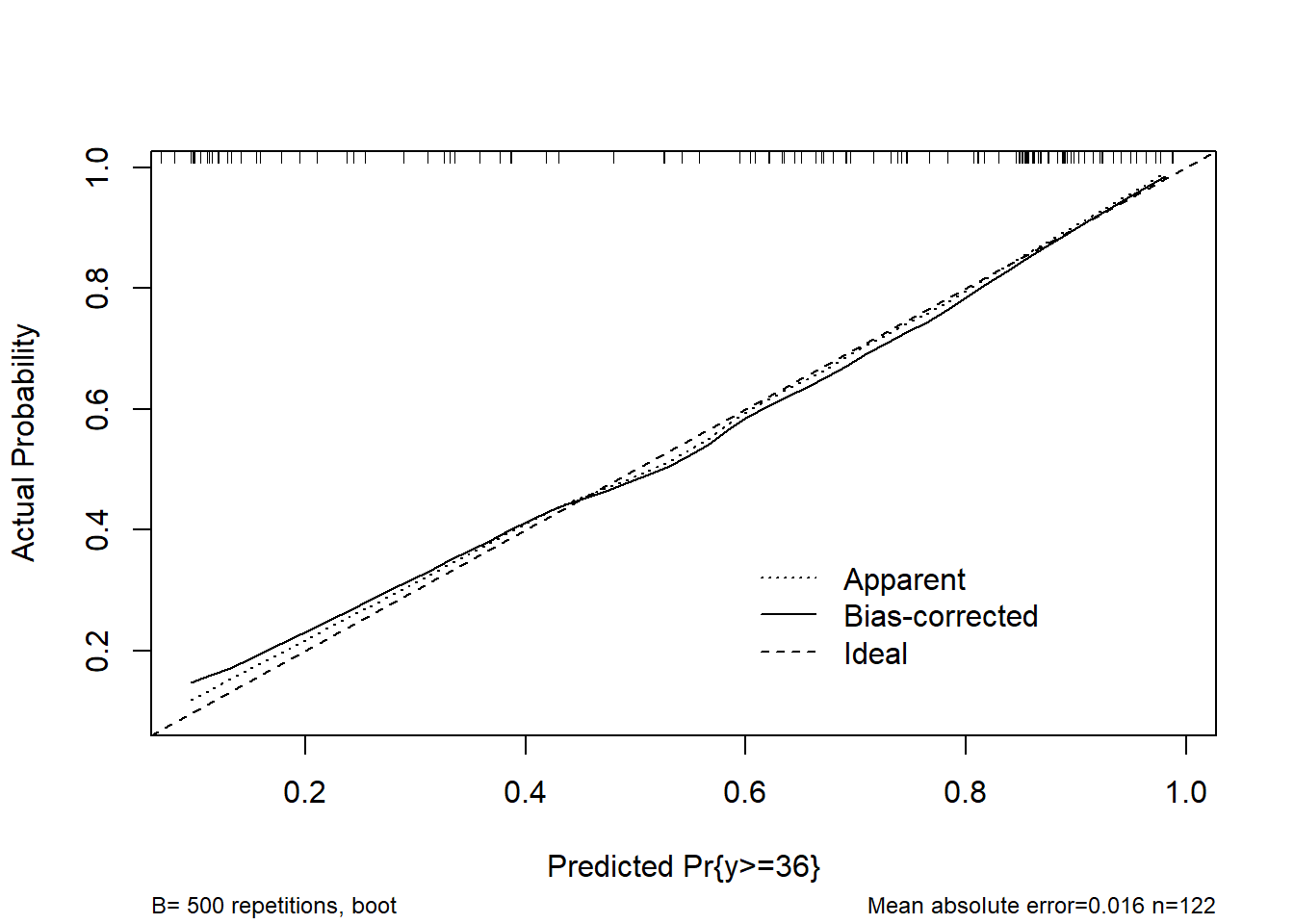
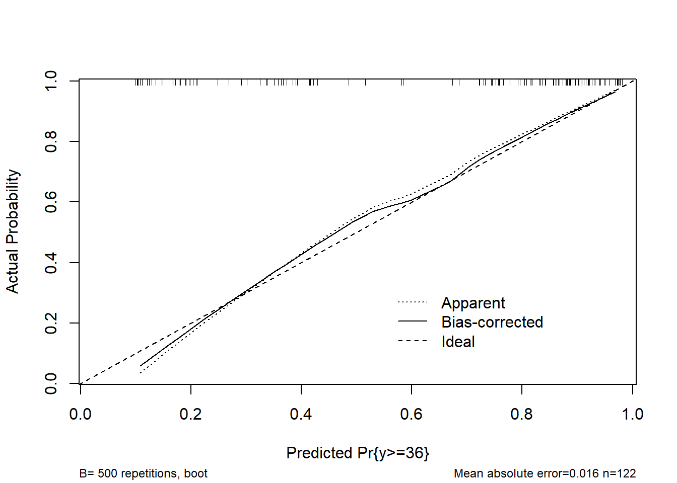
calibrate(f, method = 'boot', B = 500, group = data$y) # calibration curve using boostrap
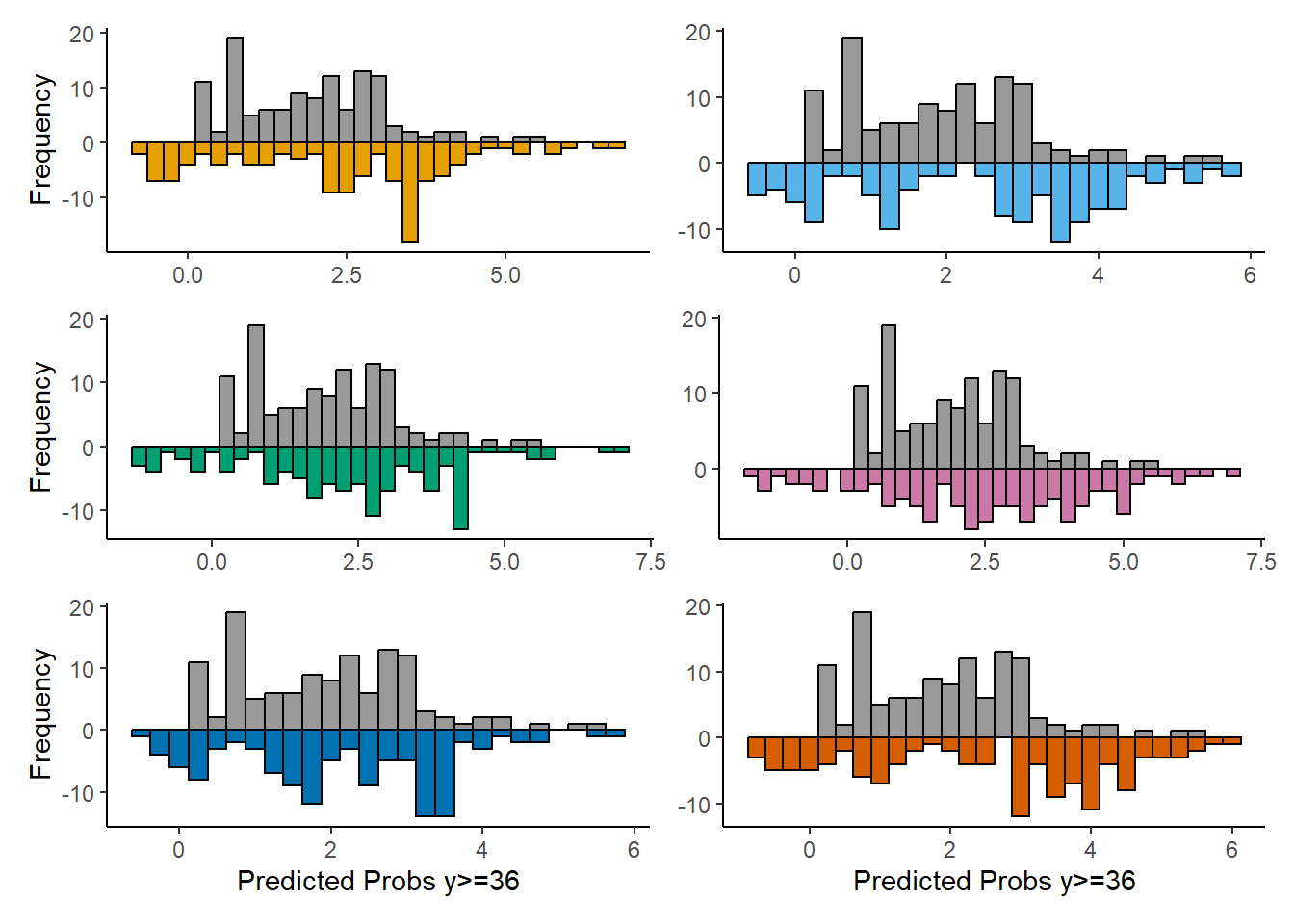
pred <- predict(f, type = 'lp', ycut = 36) # predicted probabilities for y>=36
1-var(predBase)/var(predx) # fraction of new information

• These measures are displayed on the figures attached;
• From these analyses I conclude that x4 makes the greatest contribution to increasing predictive power of the Base Model;
• x1 and x2 are much simpler/quicker tests to perform in clinical practice, and they also seem to be important for predicting y (either in isolation or combined), but their performance indexes are a bit conflicting in my view;

Any comments?

[f2harrell]

Not sure this is posted in the right topic. Should have probably been in RMS Multivariable Modeling Strategies - modeling strategy - Datamethods Discussion Forum

You are going to way too much trouble for the goal you have. Add all of those variables at once and do a likelihood ratio chunk \chi^2 test for added value. And describe the added value using a type of partial R^2 measure. And compute the proportion of log-likelihood explained by the new variables. See also Statistical Thinking - Statistically Efficient Ways to Quantify Added Predictive Value of New Measurements

[FurlanLeo]

Thank you Professor.
Ok, I will move the post then.

Actually, my analysis is based exactly on this. That’s why I made the back-to-back histograms and the fraction of new information plot.

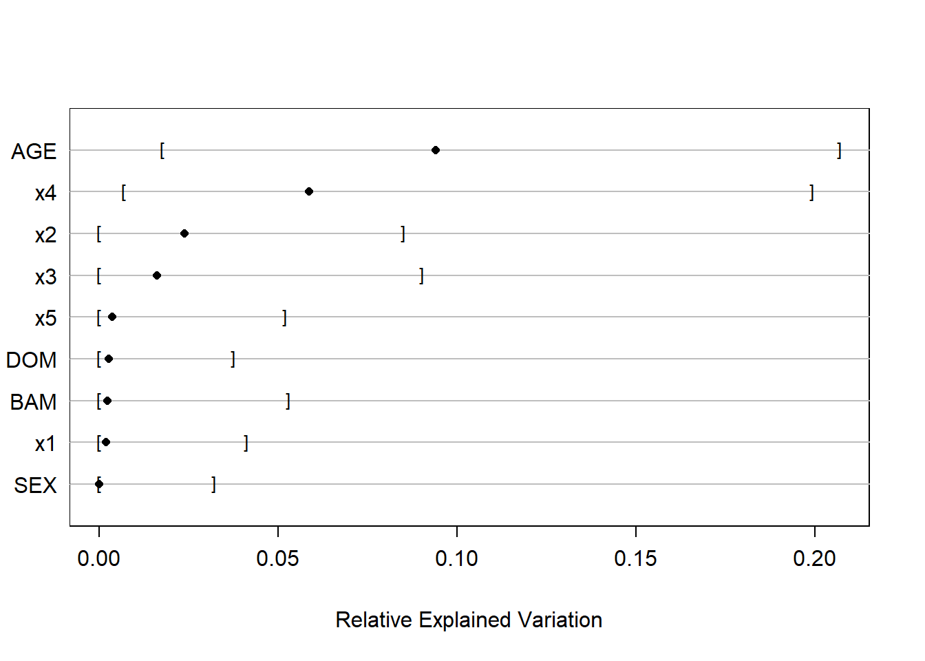
So it’s better to have a full model with all the xs in and then compute e.g., Proportion of Overall Chi-Square and then Relative Explained Variation using bootstrap, as shown in Section 5.1.3 of RMS?

[f2harrell]

Don’t need to move the post, just keep in mind for next time. Yes to your questions. The upcoming version of rms has the rexVar function which automatically incorporates bootstrap repetitions if you’ve run bootcov, to get uncertainties in a new relative importance measure. The rms course notes are already updated to include an example of this.

[FurlanLeo]

Thank you Professor!

Here are the results of my updated analysis.
Please, any comments or suggestions for improving it?

1. Chunk test / likelihood ratio chi-square test for added predictive value of the clinical measures altogether:

#   Chi-Square         d.f.            P 
# 6.386165e+01 7.000000e+00 2.545708e-11

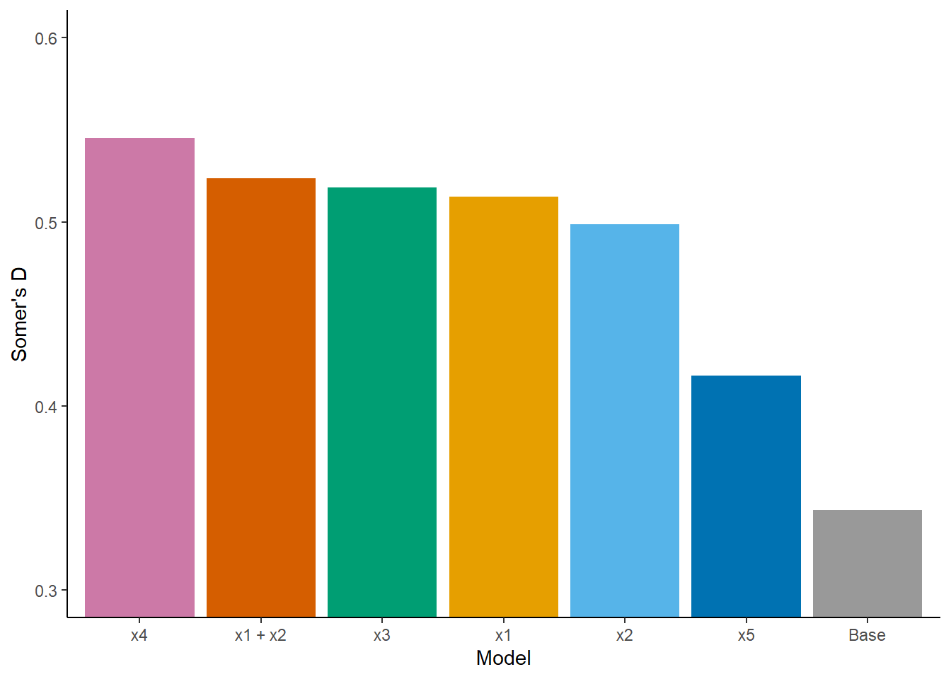
2. REV (500 bootstrap resamples of the full model):
   

   

3. Fit x4 model:
   lrm(formula = y ~ DOM + BAM + SEX + rcs(AGE, 3) + rcs(x4, 3),
data = data, x = T, y = T)

4. Anova (Likelihood Ratio Statistics):
   Significant association of AGE (df=2; p=0.0007) and x4 (df=2; p<0.0001)

5. Bootstrap model and partial effects plots:
   

   

6. Model validation with bootstrap (B=500):
   Somer’s D (corrected index) = 0.5455

7. Model calibration with bootstrap (B=500):
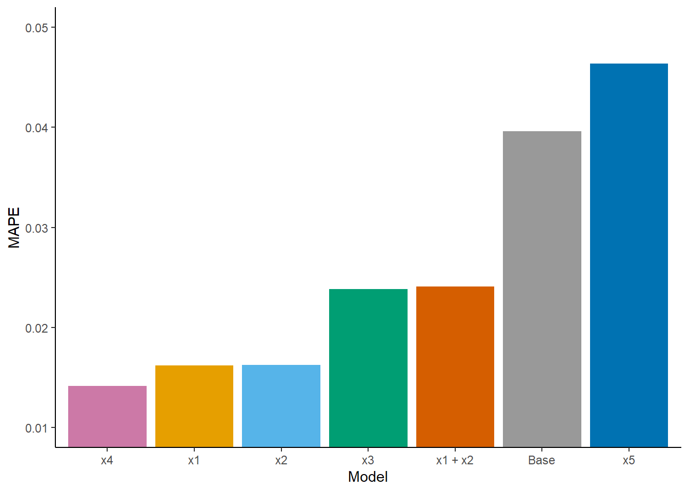
   Mean absolute error = 0.014
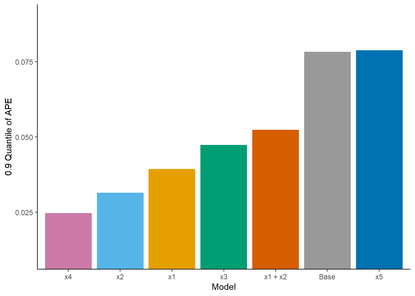
   0.9 Quantile of absolute error = 0.025
   

   

8. Nomogram:
   

   

[f2harrell]

Nice work. I don’t think of any suggestions.

[FurlanLeo]

Thank you Professor, I appreciate the feedback.

I just want to make sure I got this right…

The REV approach is much more straightforward, but is the other approach wrong (Question 1)?

By other approach I mean when I fit a base/ reference model and a separate model for each new predictor (i.e., base model + new predictor) and then compare these models in terms of their predicitve performance, using discrimination, calibration and prediction error indexes, e.g., D_{xy}, E_{max}, Mean Absolute Prediction Error, etc.

If this approach is correct, then what would be the most appropriate index for choosing the best model (Question 2)? The reason I ask is because sometimes these indexes are in disagreement, e.g., for index a, model w is the best, but for index b, model z is the best.

Section 4.10 from RMS contains a list of criteria for comparing models. If I undestood correctly, calibration seems to be the most important criterion if the goal is to obtain accurate probabilities for future patients, whereas discrimination is more relevant if we want to accurately predict mean y.

This matters to me beacuse in my case (PO models fitted with lrm) y has 35 intercepts and all the bootstrap validations and calibrations are performed using the middle intercept, but from a clinical perspective I think it is more relevant to predict mean y. Does that mean I should focus on discrimination (Question 3)?

Finally, considering the recommendations on section 13.4.5 from RMS, when describing my selected best model, besides presenting partial effects plots and a nomogram, both on the mean scale, what else could I do (Question 4)? I think it could also be relevant to report predictions (on the mean scale and with confidence limits) for new subjects using expand.grid and predict.lrm. But I’m having trouble with the arguments of Mean.lrm:

new <- expand.grid()
m <- Mean(f, codes = T, conf.int = T) # what about the design matrix ‘X’ (Question 5)?
lp <- predict(f, new)
m(lp)

Thank you for your time Professor.

[f2harrell]

Concerning model comparison I would not use that approach but would rather use the approach here. This emphasizes the gold standard log likelihood-based measures plus measures built on dispersion of predicted values on the linear predictor or probability scale. Don’t fit separate models for “each new predictor” as this is too similar to stepwise regression. Pre-specify 2-3 models for the competition.

This leaves the question of when to consider calibration. Usually I demonstrate good overall calibration in the final, single, model.

[FurlanLeo]

Ok Professor,
Thank you very much for the valuable suggestions.

[FurlanLeo]

Hi Professor @f2harrell,

One final question that remains on this analysis approach (https://discourse.datamethods.org/t/rms-describing-resampling-validating-and-simplifying-the-model/4790/137?u=furlanleo):

I understand that the Relative Explained Variation index, computed by rexVar, should only be used in a final, pre-specified model, and not for selecting important predictors.

Therefore, I believe there’s a problem with my approach from above, where I first do a chunk test for the added predictive value of 5 new measures (X1, X2, … X5) and then, after confirming that there is indeed added predictive value, I use rexVar to decide which of these 5 new measures is more important, and finally I select this more important measure (e.g., X4) to build my final model.

If that is the case, then I think a better approach would be to first select 3 of the 5 new measures and build a separate model for each, and then use AIC to compare these 3 models and select the best one to be my final model:

• Model 1: y ~ DOM + BAM + SEX + rcs(AGE, 3) + rcs(X4, 3)
• Model 2: y ~ DOM + BAM + SEX + rcs(AGE, 3) + rcs(X1, 3)
• Model 3: y ~ DOM + BAM + SEX + rcs(AGE, 3) + rcs(X2, 3)

Is my understanding correct?

I think this is in line with the idea that, if the sample size is not large enough, then selecting winners is a futile task, as shown in the “boostrap ranking of predictors” example here.

Thank you.

[f2harrell]

No that is not correct. Just pre-specify the model, allowing for as many parameters as you think may be needed, subject to limitations imposed by your effective sample size for Y.

[FurlanLeo]

Sorry, I don’t think I expressed myself well.
Could you kindly have another look at what I did here?

You said afterwards that it was a “nice work”, but I’m confused because after confirming the added predictive value of the 5 new measures altogether, I did a REV analysis using rexVar and decided that X4 was The Best measure among the 5, and then I built my prediction model with X4 only (besides the “base” predictors). Isn’t that a bit like variable selection?

That’s why I mentioned in my last post that it was my understanding that rexVar should only be used in a final model (but not to specify this final model).

So the big question is: what to do when you want to select, among a set of new clinical measures, only one measure to include in your prediction model?

I’m aware that I should preferably be fitting a full model with all the measures in (possibly with some form of penalization) and then using such model as my new prediction model. But the central ideia is to choose among the new measures only one, as using all of them in clinical practice would be too laborious. Is that reasonable?

Thank you!

[f2harrell]

Just like when running anova(), the fact that you want to quantify which predictors are very important doesn’t mean that should lead to changes in the model. You are getting into the classic Grambsch-O’Brien problem discussed in RMS.