@Tripartio GLM does not assume linearity so I am not comfortable with the framing of the question. And beware of “average effect” as the estimated effects are conditional on other predictors and on the interaction being zero. Partial effect plots can replace coefficients in a sense, if there are no interactions or the interactions are with discrete variables (or there are 2 continuous variables interacting and you make a 3D graph, which can be hard to estimate predicted values from).
Thanks @s_doi and @f2harrell for your responses. But isn’t the issue about interactions exactly the same with coefficients? Aren’t GLM coefficients likewise only meaningful “if there are no interactions”? That is, I do not see partial effect plots as a disadvantage compared to coefficients in this sense–they just share the same caution.
Your framing of the question makes it seem as if partial effect plots are a stand-alone method for estimating a relationship between a predictor X and an outcome Y, but they’re not. Partial effect plots are just visualizations of quantities calculated from a fitted model. In fact, the reliance of a partial effects plot on a particular fitted model is right there in the rms code you wrote: ggplot(Predict(model)). So it’s not true that “partial effects plots…visualize relationships of any shape with no need to assume the distribution of the X or the Y variable”. The visualized relationships in the plot will reflect whatever assumptions you made in your model. The relationship it shows between the predictor and the outcome will capture the true relationship only to the extent that the underlying model does. And, as Frank mentioned, GLMs do not assume linear relationships between predictors and outcomes, and can in fact incorporate flexible modeling of non-linear relationships via restricted cubic splines.
In addition to that excellent reply, it’s helpful to think more generally than main effects and interactions and to assume that interaction effects are carried along into any estimate that is meaningful.
@Tripartio, you have hit upon an important point here. When a predictor X is associated with multiple terms in the model (e.g. because of interactions or modeling via polynomials or splines), then the individual coefficients may no longer correspond to meaningful quantities by themselves. Instead, meaningful quantities might only emerge when we consider multiple coefficients at a time. That is where things like plots of predicted values can be much more informative about the relationship between X and Y than say a table of estimated regression coefficients.
1 Like
And chunk tests, e.g. testing whether one predictor interacts when any of three other predictors, are appropriate.
Good Afternoon Professor Harrell and everyone! It’s awesome to be here. I 've currently making my way through RMS and Flexible Imputation to really round out some material I wasn’t exposed to in undergrad and graduate statistics.
Currently, I am trying to build a diagnostic model on case controlled data. Specifically-I am having issues with some missingness structure, as well as some data that I believe is redundant and needlessly increases the dimensionality of my sample space. I’d like to build a few competing models after imputing and performing redundancy analysis. Our primary goal is a predictive model, so I have been following RMS Chapters 4 and 5 in this regard.
My thoughts on how to proceed without falling into some of the pitfalls that produce over-optimistic models is the two step process below. I have been wrestling with the though that including all steps within the same ‘double bootstrap’ loop is better-but I fell like I need to account for uncertainty in MI + RDA step before any modeling validation and selection is done.
-
Redundancy Analysis + MI
- Create M Imputed Datasets (Using FCS/Additive Regression with PMM as an example)
- For Each Data Set, fit flexible parametric additive models to the data (Using redun or the like)
- ‘Pool the results’ of the RDA by looking at the relative frequencies the i-th predictor is included in
the selected set of predictors - Establish a minimum threshold for the frequencies in part 3 to discard from the original data.
Here I’m a bit confused how to establish a threshold that will generalize well - Discard any variables that do not meat the threshold in the original data
-
Model Validation and Selection:
- Start with the original (non complete) data-but screen out the predictors that were found by step
(5) above. - For each model i = 1,2…,I:
- For m = 1,2…,M:
- Fit model i to Imputed Data set M
- Bootstrap Validate fit as in 5.3.5 in the online text
- Average the M apparent performance estimates over the imputations for model i to get an
apparent performance for model i, S_{iapp}
- Get Generalized Performance Estimates:
-
For Imputed Data sets 1,2,…,M
- For resamples j = 1,2,…J
- For Each Model i = 1,2,…I
1. Fit model i to the j-th resample of dataset M
2. Calculate the performance estimate S_{ijm_boot}
3. Calculate the additional performance estimate S_{ijm_orig}
- For Each Model i = 1,2,…I
- For resamples j = 1,2,…J
-
For each of the M imputed datasets that now have bootstrap estimates of performance:
- calculate apparent optimism for model i which is (forgive my lack of markdown knowledge 1/j*SUM(S_{ijm_boot} - S_{ijm_orig))
- Average the apparent optimism for model I over all imputed Data sets for; O_{i}
-
Calculate Optimism of apparent Imputed Performance Estimates:
- S_{i_adj} = S_{iapp}- I_{I}
-
- Start with the original (non complete) data-but screen out the predictors that were found by step
Am I correct in my approach here? Please let me know how I can elaborate more if needed, and please forgive the markdown-I’d be happy to fix if necessary.
For Reference: I have used this post here to guide my thinking.
Thank you so much!
I don’t think I can digest all that in one go. I’m not a fan of the “select features that are selected in >= x% of bootstrap samples” approach. And redun doesn’t seem to git rid of enough variables in many cases. Another thought is that sometimes when running a multi-step approach it is better to stack all the imputed datasets and run the procedure once on the stacked dataset, being careful to emphasize point estimates (which are helped by duplication) and not standard errors (which are artificially low because of duplication).
Good Afternoon Professor! Thank you for the reply.
Please let me know how I can better frame the approach-my notion was a bit lacking thanks to some markdown unfamiliarity… I’d be happy to elaborate more on the problem if that helps. My Approach above is really just to make sure that probably capturing the uncertainty present in the redundancy analysis prior to any selection through redun (I’ve been careful in eliminating prior features using apriori knowledge and DAGS) and then account for uncertainty in model selection with imputation (sadly on a dataset that is not especially large=approx. 5000x20, but some of the variables are factors with many levels so closer to 5000 x 50),. I’d like to build my foundation a bit more so I can (hopefully) begin to move the needle in terms of ‘not discarding inference for prediction’ that’s becoming more common in industry.
Yes, I completely understand why you’re not a fan of the 'remove features that are selected in x% of bootstraps"-I think you demonstrate the unreliability of selection really well in your printed text of RMS (and you’ve helped me fix some bad habits through this!).
As this problem is primarily prediction (I’m working to get our team out of the predict to learn rut)-I really think stacking is an option. As a follow up to being able to readily obtain a point estimate for say-the g index or R^2, would you say that the empirical bootstrap to compute the standard error of the variance in performance metric is of some use (my thoughts are that it will be too narrow)?
I’m curious if you’re doing anything to account for the case-control study design?
On the main question there are conflicting opinions in the literature about whether unsupervised learning steps need to be repeated afresh within resampling loops. It is good to at least do a few separate iterations showing the degree of stability of the unsupervised learning procedure whether or not you incorporate this instability in the final outcome model.
When an unsupervised learning precedure is unstable, it is unstable in a way that does not systematically hurt or benefit the final outcome model. So an easy way out is to rationalize not repeating the unsupervised learning but to do it once outside the main validation loop. I hope someone will do more simulation studies to inform us about best practices.
2 Likes
Esteemed Members !
My model is Ordinal Logistic Regression Model
I visited the help of rms::validate.lrm() and found 3 things to note:
(1) Examples used “boot” but not “crossvalidation” method with recommendation of B = 300. Is there a reason why not to use “cross” method ? If it is OK to use it, what is the recommended value of B?
(2) I have an ordinal outcome with 4 classes. the “help” recommends that “In the case of an ordinal model, specify which intercept to validate. Default is the middle intercept.” Thus, I wrote the validation function as detailed below with kint = 1,2,3
(3) I used the Dxy.method = “lrm” as it is an ordinal model (not binary)
# validate.lrm {rms}
?rms::validate.lrm()

# normally B=300

# In the case of an ordinal model, specify which intercept to validate.
# Default is the middle intercept.

validate(fit = model, method="boot", B=300, kint=1, Dxy.method ="lrm")
validate(fit = model, method="boot", B=300, kint=2, Dxy.method ="lrm")
validate(fit = model, method="boot", B=300, kint=3, Dxy.method ="lrm")
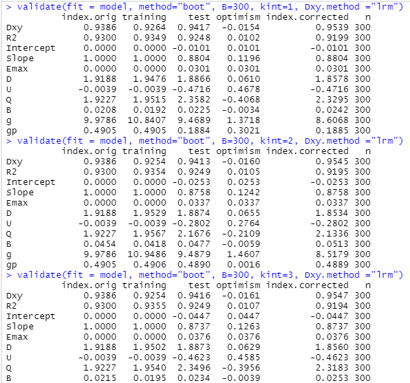
This was the output for kint = 1,2 and 3
My Questions
(1) Is there a better / optimum way to write the validation function ?
(2) Is it acceptable that the optimism is -ve and thus the corrected Dxy is greater than the original Dxy ?
(3) What type of R-squared was reported in this output. I don’t think it is Nagelkerke’s?
Excellent work. The only reason to run with different kint is to get indexes like the Brier score which combine calibration and discrimination, so depend on the absolute predicted values unlike measures of pure predictive discrimination.
The bootstrap is generally recommended unless the overfitting is extreme (effect sample size not much larger than the number of parameters). Use B=500 to be confidence but the actual B depends on the sample size (larger samples sizes require smaller B but never hurts to overkill).
The default Dxy.method is already lrm for an ordinal model with > 2 levels of Y.
You don’t usually see Dxy get larger but you have an exceptionally high signal:noise ratio. Make sure that no feature selection was done before the validation step as you didn’t inform the validation algorithm of any feature selection that needs to be repeated afresh at each resample.
1 Like
Second time in one Quarter ! I am the luckiest Biostatistician alive. ![]()
2 Likes
I have noticed that my prognostic model has better discrimination in the test set vs the training set for long term follow up overall survival (10 yrs) [AUC = 0.786 vs 0.773, respectively], whereas the discrimination is lower in the test compared to training set for short term follow up (3 yrs) [AUC = 0.799 vs 0.801, respectively]. Is this normal in cox regression based predictive models? Here are the codes I used to fit the model in the training set and also to validate this in a test set.
#fit1 using training set (5 variables included in the model)
fit1 ← cph(Surv(futime, death) ~ x1+ x2 + x3 + x4 + x5, data = Train, x = TRUE, y = TRUE, surv = TRUE)
#validation
Test$predicted ← predictrms(fit1, newdata=Test,
se.fit=FALSE, conf.int=FALSE,
kint=1, na.action=na.keep, expand.na=FALSE,
ref.zero=TRUE)
#AUCs
ROC.obj ← roc(Test$death, Test$predicted)
auc(ROC.obj)
ci_aucTrain ← ci.auc(ROC.obj)
ci_aucTrain
I just wanted to ask if by saying it is difficult to get c-index below 0.5 you also mean it is possible? I am asking because I have observed that one of my biomarkers had an individual c-index of 0.46.
Use the validate function that is for cph models to get strong internal validation, which is better than “external” validation unless both training and test samples are very large. You’ll see negative D_{xy} correlations with Cox models (c < 0.5) because high X\beta \rightarrow shorter survival, so we negate D and typically get c > 0.5. But even then c is possible to be < 0.5 (“predictions worse than random”).
Thank you so much, I get your point that this is for internal validation where I do not have large train and test datasets.
Yes, the non-huge N situation is where you don’t have the luxury of splitting the data.
Much appreciated and thank you.