I found that the HRs obtained from summary(cph) are quite different to the ones from coxph. I read that coxph gives HR for a one unit increase and cph for an interquartile range increase.
1.) How can I obtain HRs for a one-unit increase using cph function as with the coxph function? I believe that I could use HR for one unit increase = exp(beta-coef), where the beta-coef is extracted from the output of cph (not summary(cph)) since this should be the beta-coef for a one unit increase.
Is it correct that the displayed effect in summary(cph) is the beta-coef or HR for an increase in interquartile range?
Is there a way to change the summary(cph) to display HRs by one unit increase?
2.)
Using summary(survfit(coxph_model),time=5)$surv, I can obtain the baseline survival probability at 5 years.
Is there a function for this in rms?
You’re right about the default for summary.rms being interquartile-range effects. You can get any effect estimates you want using things like
dd <- datadist(mydata); options(datadist='dd')
f <- cph(...)
summary(f, age=c(20, 21))
summary(f, age=c(30, 31))  # same as above if age modeled linearly
contrast(f, list(age=21), list(age=20))
For your second question, the function you need in rms is survest.
survest allows you to specify covariate settings at which to predict. For ones you don’t specify the default is the median or mode. Try getting specific predictions (i.e., at specific covariate values) for both functions to make sure they agree.
Greetings all. I have a process question. I am working with others to create a risk prediction model for a binary outcome in a large registry with missing data. We used MICE to impute the missing data, then the ‘fit.mult.impute’ function in ‘rms’ to run the logistic regression using the imputed datasets. We then did internal validation using bootstrapping of this process. Given a little overfitting, we are interested in doing uniform shrinkage of our regression parameters using the bootstrapped calibration slope value. Question is, we cannot find methods to reasonably perform the shrinkage across the imputed datasets. I welcome any and all thoughts on this approach. Thanks in advance.
I was wondering if you would not mind answering a question for me regarding the possibility of centering/setting a referent group in restricted cubic spline analysis?
I have an exposure, that I want to conduct restricted cubic spline analysis for its association with a time-to-event outcome. I’ve been successful in conducting the RCS model, but I wanted to set the number of hours (7 – 8) as my referent group for restricted cubic spline analysis.
How could I manipulate my R code (shown below), to set the Hazards Ratios for two values of my exposure to 1.0? I want a range of my exposure values (7 - 8) to be the referent rather than a single point (7 or 8).
Welcome to datamethods Noah. You code is not using the rms package. The solution to your problem using rms is to think of reference values as arbitrary when fitting the model, then getting any effect of interest after doing the fit. There are two main ways of doing this: (1) using summary (long name summary.rms) to get effect ratios, or (2) using contrast (long name contrast.rms) to do this. contrast gives the most control. Here’s a sketch:
dd <- datadist(mydata); options(datadist='dd')
f <- cph(Surv(dtime, event) ~ rcs(exposure, 4) + x2 + x3, data=mydata)
contrast(f, list(exposure=4), list(exposure=1))   # log hazard at 4 hours minus 1 hour
contrast(f, list(exposure=1:20), list(exposure=1))  # 20 differences, one of them zero
You can put the output of contrast into another object and then plot it.
Thank you so much Dr. Harrell. With respect to datadist(), could you tell me what exactly this function is doing? When I run the code provided (with slight alterations to match my data)
dd = datadist(mydata)
options(datadist=‘dd’)
I receive an error message after attempting to run the contrast statement above:
Error in Getlimi(name[i], Limval, need.all = TRUE) :
no limits defined by datadist for variable newsleepduration
Is the datadist() option meant to include my entire dataframe?
datadist stores default values for prediction, effect estimation, and adjustment reference values. It’s best to run it on the whole data frame. If you add a variable later you’ll need to add that, e.g. dd <- datadist(dd, newsleepduration).
Hi,
I’m trying to draw a calibration curve for a validation cohort using rms package. A Cox model was fitted for the development cohort. I have seen in a few papers; Development and validation of a simple-to-use clinical nomogram for predicting obstructive sleep apnea | BMC Pulmonary Medicine | Full Text https://clincancerres.aacrjournals.org/content/27/12/3414 authors have created calibration plots for both development and validation cohorts.
I could understand how to create the calibration plot for the development cohort using the general calibrate() function in rms. But, I’m not too convinced about how to draw the calibration plot for the validation cohort. Would this be from the Cox model only using the linear predictor (prognostic index) for the validation cohort? or could someone let me know any place to look for this?
Be sure that your testing and development cohorts are from different times, countries, or from drastically different types of patients. Otherwise you are in all likelihood doing internal validation and split sample methods are unstable unless N > 20,000 for example.
For a real external validation of absolute predictive accuracy (calibration), use the rmsval.surv function whose documentation may be found here. Note that you can specify either a cph fit object or the actually estimated probabilities to val.surv. Raw data from the validation cohort is specified using newdata.
Thank you for your reply. After searching more on this, I found this discussion on your platform: Calibration of Cox model - #11 by lif. I think this uses the approach that you have mentioned in your reply. Is that correct?
Yes that is a good example of what I referred to. In this case it’s for a parametric survival model; a minor change would make it work for the Cox model.
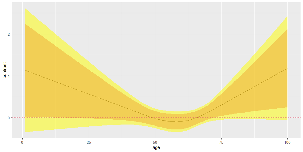
I am trying to do interaction plots for the treatment by a continuous baseline covariate interaction in analyzing time-to-event endpoints. My main problem is how to get a simultaneous confidence bands. I was able to successfully implement it in rms, but the plot is on the log(HR) scale and apparently the fun = exp argument for the contrast() function does not do the transformation to the HR scale. Is there any way of applying the exp transformation to get the plot on the HR scale with its confidence band?
The code with the output is below.
library(survival)
library(rms)
data(cancer)
dat ← colon
dat$sexC ← ifelse(dat$sex==1, “F”, “M”)
fit ← cph(Surv(time, etype) ~ sexC * rcs(age, 3), data = dat)
M ← contrast(fit, list(sexC = ‘F’, age = 1:100), list(sexC = ‘M’, age = 1:100), conf.type = “simultaneous” , fun = exp)
M0 ← contrast(fit, list(sexC = ‘F’, age = 1:100), list(sexC = ‘M’, age = 1:100), fun = exp)
Dear Experts:
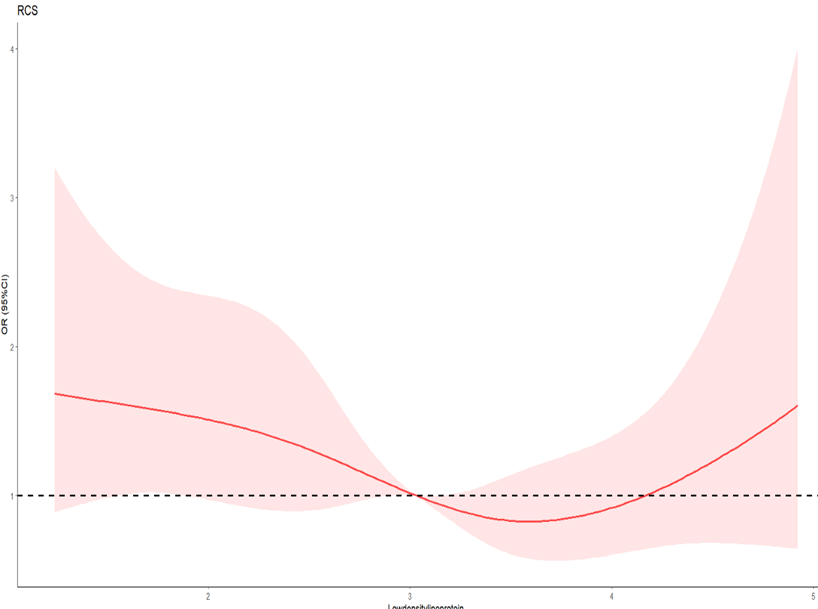
I am working on a study using ordinal logistic regression. The dependent variable (Y) was set to 4 levels, from None to Severe. I want to use restricted cubic splines to explore their potential nonlinear relationship. Based on my limited knowledge of the rms package, I wrote the following code.
The weights were obtained based on the previous propensity score. However, there is always an error here which is very confusing to me
“currently weights are ignored in model validation and bootstrapping lrm fits”
I would like to ask how can I handle this situation.
I also tried the rep() dunction, While it works, I can’t guarantee its results are correct. Also, I noticed that the weights used by lrm and all the weights in svyolr do not present the same point estimate and 95%CI (but are numerically approximate), is this normal?
For example, The OR vaule obtained from svyolr is 0.79 while in lrm is 0.62. After i tried to plot the lrm model (Of course I ignored that error, I think it might not be right) The export rcs curve presented as follows:
I answered your question in the code below and gave some coding suggestions also. Be sure to use ← instead of ← next time, and change quotes to R-compatible quotes or the code won’t execute.
library(survival)
library(rms)
data(cancer)

dat <- colon
dat$sexC <-  ifelse(dat$sex==1, 'F', 'M')
# dat <- transform(dat, sexC=ifelse(...)) or
# dat <- transform(dat, sexC=factor(sex, ...))

fit <- cph(Surv(time, etype) ~ sexC * rcs(age, 3), data = dat)

M <- contrast(fit, list(sexC = 'F', age = 1:100), list(sexC = 'M', age = 1:100), conf.type = 'simultaneous' , fun = exp)
# Type ?contrast.rms to see documentation.   You'll see that fun= applies only to
# the print method of contrast, and to Bayesian model fits

M0 <- contrast(fit, list(sexC = ‘F’, age = 1:100), list(sexC = ‘M’, age = 1:100), fun = exp)

# Drop fun=exp and modify this example from the help file:
# Plot odds ratios with pointwise 0.95 confidence bands using log scale

k <- as.data.frame(M[c('age', 'Contrast','Lower','Upper')])
ggplot(k, aes(x=age, y=exp(Contrast))) + geom_line() +
   geom_ribbon(aes(ymin=exp(Lower), ymax=exp(Upper)),
               alpha=0.15, linetype=0) +
   scale_y_continuous(trans='log10', n.breaks=10,
               minor_breaks=c(seq(0.1, 1, by=.1), seq(1, 10, by=.5))) +
  xlab('Age') + ylab('F:M Hazard Ratio')
############################
The warning message documents that weights are not implemented in resampling validation methods in the rms package. I don’t know of anyone who has implemented this but a search of CRAN may find something.
To get to the bottom of the disagreement between the two estimation methods (rms::lrm aind svyolr) would require a lot of digging. The first thing I suggest trying is simulating data using integer case weights that can easily be analyzed by duplicating observations the number of times equal to the weights, and comparing results (in both functions) to weighted estimates on the shorter dataset and unweighted estimates on the longer dataset.