Oh woa, the problem is that there is a patient in my data having OS time less than 0 (month). Sorry, this is my fault, Prof. Harrell.
How to interpret the internal validation results in rms? What are the things that we should look for?
validate(cox.tox.3, method = “boot”, B = 500)
index.orig training test optimism index.corrected n
Dxy 0.3221 0.3378 0.3151 0.0227 0.2994 500
R2 0.2821 0.3020 0.2601 0.0419 0.2402 500
Slope 1.0000 1.0000 0.8747 0.1253 0.8747 500
D 0.0370 0.0403 0.0336 0.0067 0.0303 500
U -0.0006 -0.0006 0.0016 -0.0022 0.0016 500
Q 0.0376 0.0409 0.0320 0.0089 0.0286 500
g 0.8315 0.8728 0.7634 0.1094 0.7221 500
What are the things that we should look for?
Hi, definitely the thing you need to consider is the C-index (Concordance index). Mathematically, you can calculate the C-index by using the value of Dxy at the column index.corrected
this may seem off topic but im very interested in how methods come in and out of favour - your book doesnt seem to mention restricted mean survival (i dont have it to hand but checked the index on amazon), dave collett’s book on survival analysis also doesnt mention it + the use of the acronym rms for “regression modelling strategies” when it could be confused with “restricted mean survival” … these things suggest the sudden popularity of the latter? the original paper on rms is from the 1940s i think but new papers are appearing asking how to choose tau: On the empirical choice of the time window for restricted mean survival time Is it just me or it achieved widespread statistical approval suddenly?
That’s a terrific question and one I’ve been thinking a great deal about. First of it the link above links to a preprint dated 2020. Has the paper not been published by 2021?
For a long time I did not like residual mean life as a solution to non-proportional hazards. I’m changing a bit but would you mind moving your post to https://discourse.datamethods.org/t/restricted-mean-survival-time-and-comparing-treatments-under-non-proportional-hazards where I’ll respond? And please add something to it when you move it related to the preprint status if you can find that out. Thanks.
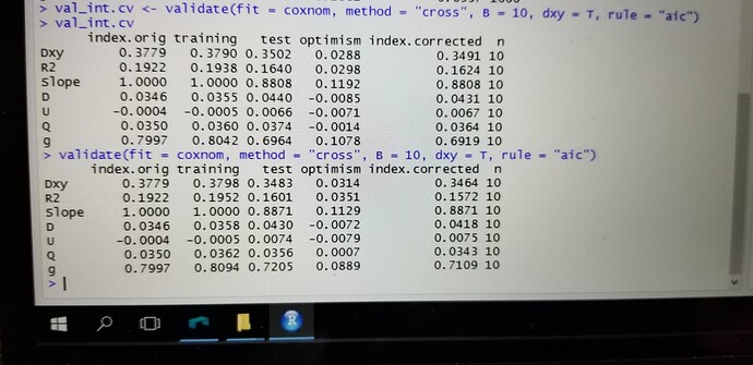
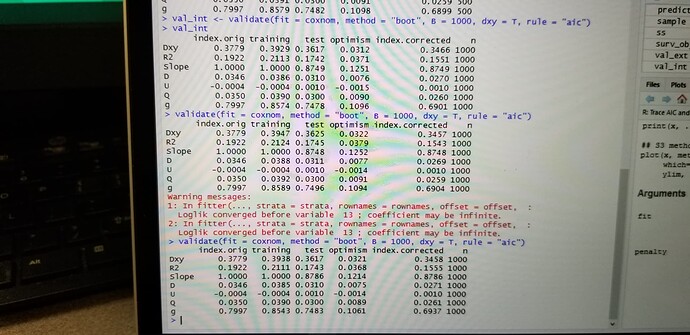
Hi, I have been trying to perform a resampling validation of a cox model using bootstrapping and 100 repeats of 10 fold cross validation. I am little surprised that with the fact that results are different with two repeated iterations of bootstrapping or two repeated iterations of cross validation. Could you explain why is this variation?
I would expect that 100 repeats of 10-fold cv should be stable. How much did results differ? If you did 1000 bootstrap reps I would also expect stability. Please give some of your results.
Prof Harrell,
I have shared a screenshot for the variation in the results despite setting the seed. Ufortunately I can’t copy paste the code…Please rectify me if there is an error in my code.
I have one more question…How can I calculate the riskscore of each individual of a cohort from a Cox model which was fitted for the entire cohort? Does the predict function give us a riskscore?
The kind of variation you are seeing from resampling (boot and cv) is what I’d expect for non-huge sample sizes. But I think you are doing only one repeat of 10-fold cv. You can increase the number of iterations for both boot and cv if you want less variation.
To get predicted log relative hazards (linear predictors; scores) or survival probabilities you can use predict, Predict, survest. To get the formula for the linear predictor use Function or latex.
Thank you very much for both the answers Prof. Harrell.
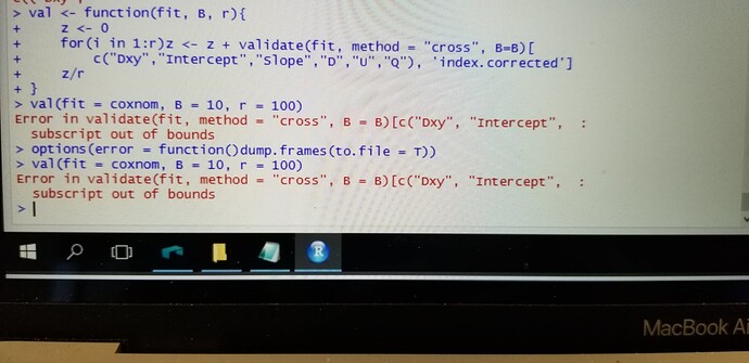
However, I was wondering how I can increase the repeats of 10 fold cross validation. I was looking through your course notes and I could not find it. I am sure that it is my fault or my lack of knowledge.
Along these lines for cv:
## Function to do r overall reps of B resamples, averaging to get
## estimates similar to as if r*B resamples were done

val <- function(fit, B, r) {
  z <- 0
  for(i in 1:r) z <- z + validate(fit, method='cross', B=B)[
          c("Dxy","Intercept","Slope","D","U","Q"),'index.corrected']
  z/r
}
val(fit, 10, 100)  # 100 repeats of 10-fold
Since you are using a Cox model, remove "Intercept" from the vector of statistics names to validate.
Hello! I created a plot with odds of aneurysm rupture on the Y axis and size of the aneurysm on the X axis. To make the plot easier to understand, I was trying to find a way to convert the odds into probability of aneurysm rupture. Dr. Harrell suggested using fun=plogis. The new plot makes sense to me but I just wanted to confirm that the code is right and the Y axis is in terms of probability.
Here’s my code:
library(rms)

Xax_var<-caa11_1$size_cm
Yax_var<-caa11_1$ruptured

caa11_1$aneurysm_with_fistula[which(caa11_1$aneurysm_with_fistula== "1")] <- "Fistula"
caa11_1$aneurysm_with_fistula[which(caa11_1$aneurysm_with_fistula== "0")] <- "No Fistula"

stratifier<-caa11_1$aneurysm_with_fistula

dd <- datadist(Xax_var,stratifier)
options(datadist='dd')

f <- lrm((Yax_var) ~ rcs(Xax_var,5)+stratifier, x=TRUE, y=TRUE)
anova(f) #p value

#For odds
plot(Predict(f, Xax_var, stratifier, fun=exp), xlab="Size (cm)", ylab="Odds",
     ylim=c(0,0.45),
     xlim=c(0,8),
     main = "Aneurysm Rupture: Fistula vs. No Fistula\np=0.0036 (total), p=0.0035 (stratifier)")

#For probability
plot(Predict(f, Xax_var, stratifier, fun=plogis), xlab="Size (cm)", ylab="Probability",
     ylim=c(0,0.45),
     xlim=c(0,8),
     main = "Aneurysm Rupture: Fistula vs. No Fistula\np=0.0036 (total), p=0.0035 (stratifier)")
That all looks correct.
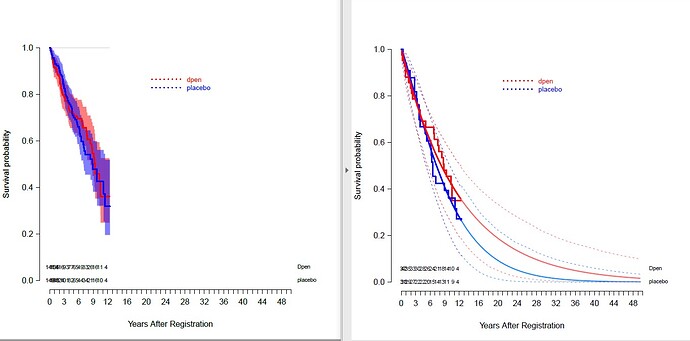
I wanted to know how to fill bands for confidence intervals in the “lines” function applied to survplot.
The left plot shows the confidence bands for Kaplan Meier curves with transparent overlap. I’d like the same for right plot for the parametric curves.
Any help would be greatly appreciated!
Christopher
code below:
# dpen is a drug
dat_dpen <- filter(dat, drug_Dpen_placebo == '1')
dat_placebo <- filter(dat, drug_Dpen_placebo == '0')

survobj_dpen <- Surv(dat_dpen$regis_to_event_d/365.2422,dat_dpen$status_cens_death == 1)
survobj_placebo <- Surv(dat_placebo$regis_to_event_d/365.2422,dat_placebo$status_cens_death == 1)

surv_dpen <- flexsurvreg(survobj_dpen ~ 1,anc = NULL,
                         dist = w)
surv_placebo <- flexsurvreg(survobj_placebo ~ 1,anc = NULL,
                            dist = w)
survobj <- Surv(dat$regis_to_event_d/365.2422,dat$status_cens_death == 1)
par(las=1)
survplot(fit  = npsurv(survobj~factor(dat$drug_Dpen_placebo, labels=c("Dpen", "placebo"))),
         #conf = c("none"),
         conf = c("bands")[1],conf.int = .95, col.fill= c(rgb(red = 1,green = 0,blue = 0,alpha = 0.5),rgb(red = 0,green = 0,blue = 1,alpha = 0.5)),
         xlab = "Years After Registration", ylab = "Survival probability",
         xlim=c(0,50),
         label.curves = FALSE,
         levels.only  = TRUE,                    # show only levels, no label
         time.inc = 1,                           # time increment
         n.risk   = TRUE,                        # show number at risk
         lwd = 2,
         lty = c(1,1),
         cex.n.risk = 0.7,
         adj.n.risk = 0,
         col = c("red","blue"),
         col.n.risk = c("red","blue")
)
legend(x=20,y=.9,bty="n", legend=c("dpen", "placebo"), text.col= c("red","blue"),
       lty=c(3,3),lwd=2,col = c("red","blue"),seg.len=5,cex=0.85)
dev.off()


# fitted to data
lines(surv_dpen,type = "survival",ci = T, xnt="n",col = c("blue"),lty= c(1),
      ci.lwd= 3,lwd = 3)
lines(surv_placebo,type = "survival",ci = T,xaxt="n",col = c("red"),lty= c(1),
      ci.lwd= 3,lwd = 3)
I’m changing the names of variables in my data frames to make them more intelligible for publication. For example I’ve changed physioDatnum to months of physical therapy. This has worked fine in general but is causing problems with both ols and stackMI. For example below aregImpute works but ols and stackMI do not. Both giving subscript out of bounds errors. Previously all these functions had worked the only difference being the column names in my dataframe. Anyone have an idea what is causing this?
s_ols <- ols(symptoms ~ `years since injury` + `age at injury` + sex +
           sports + ACLR + `months of physical therapy` + `second ACL injury` +
           `current smoker` + `subsequent arthroscopy` + `meniscus injury`,
         data = bayes_data)

mi <-
  aregImpute(∼ pain + adl + symptoms + qol + s_r + `years since injury` +
                `age at injury` + sex +  sports + brace + `months of physical therapy` +
                ACLR + `second ACL injury` +  `current smoker` +
               `subsequent arthroscopy` + `meniscus injury` ,
              data = bayes_data ,
              n.impute = 5 ,
              nk = 4,
              pr = FALSE
  )

st_pain <- stackMI(
  pain ~ `years since injury` +  `age at injury` + sex + sports + brace  +
          rcs(`months of physical therapy`, 3) + ACLR + `second ACL injury` +
           `current smoker` + `subsequent arthroscopy` + `meniscus injury`,
  blrm,
  mi,
  data = bayes_data,
  n.impute = 5,
  refresh = 25,
  iter = 5e3
)
You didn’t provide any error message. But this is not good practice. Use short variable names and provide long labels using Hmisc::label. Many Hmisc, rms, and rmsb functions use these labels in output. Define the labels in the source data frame / data.table.
From a logical point of view, using intuitively obvious variable names should be Best Practice for transparency, interpretability, code review, facial validity, and 3rd party validation.
If the technologies don’t support that, the problem is in the technology or implementations.
Using long labels helps with some of those desired characteristics of an analysis, but also add more potential places of confusion if not all of the packages/procedures used in the entire soup to nuts analysis process use & show the long labels.
Natively using sufficiently descriptive variable names is the path of Maximum Clarity and Self-Documentation, and Least Possible Confusion. (MCASDALPC, since everything needs a cryptonym.)
That said, I avoid variable names with embedded blanks. I prefer underscores but will use CamelCase if that’s the preferred naming convention of the team with which I am working.
Thank you both for your responses. I agree that clarity is important. I inconsistantly (!) switch between underscore and CamelCase while attempting to keep them short. But I admit that were someone else to read my script the meaning of the variables would not always be obvious. Beyond that my concern right now is the way that these variables appear in tables/figures which are intended for publication. In this case I’d rather not have variable names with either underscore or CamelCase.
The actual error messages are
Error in X[, mmcolnames, drop = FALSE] : subscript out of bounds for stackMI
and
Error in X[, c("(Intercept)", mmcolnames), drop = FALSE] : subscript out of bounds for aregImpute
Although I’m realizing now that stackMI needs the aregImpute output so I don’t know yet if it’s an issue for stackMI. I will try the approach Frank mentioned using labels.


