RMS Discussions

Hi Prof Harrell,

Thank you for your great R package.

I have some problems using the rms package.

  1. “datadist” in subgroup analysis;
    When performing a subgroup analysis, is it advisable to create a new “datadist” object?

For example, when performing a subgroup analysis only in male, should I do create a new “datadist” object specific to that subgroup?

ddist ← datadist(dt)
options(datadist = ‘ddist’)
cph(Surv(py, d) ~ rcs(AGE, 4),data = dt)

ddist.m ← datadist(dt[sex = m])
options(datadist = ‘ddist.m’)
cph(Surv(py, d) ~ rcs(AGE, 4),data = dt[sex = m])

  1. Use of “rcs”;
    Should “rcs” be used for all continuous variables? If not, how can I determine when to use “rcs”?
    For example, by observing plots of rcs or changes in AIC or likelihood ratios?

  2. Horizontal axis in plots of rcs;
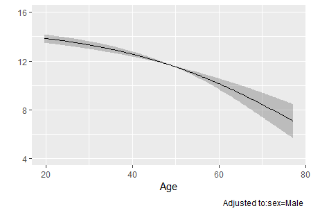
    In my data, the blood glucose range is from 0 to 100 mg/dL, but there are values above 100 mg/dL on the x-axis. I’m not very familiar with statistics; is the x-axis in the rcs plot a simulated value? It doesn’t seem to correspond directly to the actual values.

    On my rcs plot, there is a steep increase in the hazard ratio for values above 100 mg/dL . Therefore, I suspect that the risk values for this part are also speculative. Am I understanding this correctly?

I apologize for taking up your time with these simple questions; I am still learning.

Thank you.

li
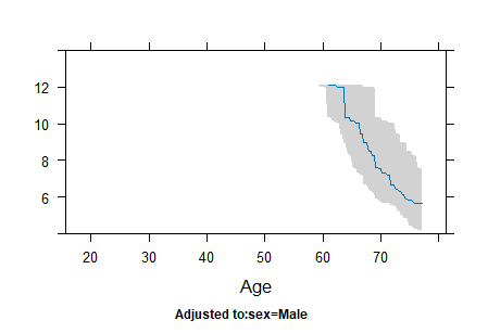
Some of your questions are covered in chapters 4 and 5 of the online notes. Pay attention to confidence bands on the plots to avoid overinterpretation. The default plots go from the 10th smallest to the 10th largest covariate values, instead of extrapolating past the data.

I don’t usually recommend subgroup analysis but instead use model-based estimates. Here you’re implying that there should have been an age \times sex interaction pre-specified. If you really want to do lower sample size subgroup analyses I would usually still use the overall datadist.

1 Like

Dear all,

Using ‘lrm’ function I recently experience the following error message:
"singular information matrix in lrm.fit (rank= 1 ). Offending variable(s): … "

Minimal reproducable example:
library(Hmisc)
library(rms)

set.seed(123)
years ← 1998:2022
prob ← seq(from = 0.01, to = 0.2, length.out = length(years))
prob ← prob / sum(prob)
date_therapy_year ← sample(years, size = 5772, replace = TRUE, prob = prob)
outcome_delir ← rbinom(n = 5772, size = 1, prob = 0.06983)
set_missing_indices ← sample(1:5772, 588)
outcome_delir[set_missing_indices] ← NA
df ← data.frame(date_therapy_year, outcome_delir)

dd ← datadist(df)
options(datadist = ‘dd’)

m ← lrm(outcome_delir ~ date_therapy_year, data = df)
singular information matrix in lrm.fit (rank= 1 ). Offending variable(s):
*date_therapy_year *
Warning message:
In lrm(outcome_delir ~ date_therapy_year, data = df) :

  • Unable to fit model using “lrm.fit”*

no problems using glm
m ← glm(outcome_delir ~ date_therapy_year, data = df)

Maybe someone can help here,
Christian

Session Info:
R version 4.3.2 (2023-10-31)
Platform: aarch64-apple-darwin20 (64-bit)
Running under: macOS Sonoma 14.2.1

Matrix products: default
BLAS: /System/Library/Frameworks/Accelerate.framework/Versions/A/Frameworks/vecLib.framework/Versions/A/libBLAS.dylib
LAPACK: /Library/Frameworks/R.framework/Versions/4.3-arm64/Resources/lib/libRlapack.dylib; LAPACK version 3.11.0

locale:
[1] en_US.UTF-8/en_US.UTF-8/en_US.UTF-8/C/en_US.UTF-8/en_US.UTF-8

time zone: Europe/Berlin
tzcode source: internal

attached base packages:
[1] stats graphics grDevices datasets utils methods base

other attached packages:
[1] rmsb_1.0-0 brms_2.20.4 Rcpp_1.0.12 lubridate_1.9.3 forcats_1.0.0 stringr_1.5.1 dplyr_1.1.4 purrr_1.0.2 readr_2.1.5
[10] tidyr_1.3.1 tibble_3.2.1 ggplot2_3.4.4 tidyverse_2.0.0 targets_1.5.1 rms_6.7-1 Hmisc_5.1-1

Fitting functions in rms sometimes use a design matrix singularity criterion that is too strict. The problem is usually fixed by add the argument tol=1e-12 or tol=1e-13 to the fitting function.

2 Likes

Wonderful, worked - thank you for the swift reply!
Christian

1 Like

Hi Dr Harrell, @f2harrell
In the help section of the cph() function, there is a segment of code plotting the median survival.

f ← cph(S ~ age + strat(sex), surv=TRUE)
g ← Survival(f) # g is a function
g(seq(.1,1,by=.1), stratum=“sex=Male”, type=“poly”) #could use stratum=2
med ← Quantile(f)
plot(Predict(f, age, fun=function(x) med(lp=x))) #plot median survival

Does this plot the median survival time for possible values of age among males?
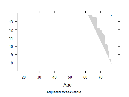
What is the reason why some age values have NA for yhat or lower or upper estimates?
image

Also, if I instead estimate the mean survival function using the Mean function, why are there estimates for yhat for the lower age ranges? Are there pros/cons for estimating median survival time versus mean survival time?

ggplot(Predict(f, age, fun=Mean(f)))
image

Finally, If I try to use the Quantile function with default median option for the survival curve with rcs for age, I’m getting a weird graph. Do you have any insights?

f ← cph(S ~ rcs(age,4) + sex, x=TRUE, y=TRUE,surv=TRUE)
med ← Quantile(f)
plot(Predict(f, age, fun=function(x) med(lp=x))) #plot median survival

image

Yes; NA arises when the follow-up duration in the data is not long enough to compute the median for the covariate combination in question.

I don’t understand why that is the case, looking at the code for Mean. When tmax is not specified and the observed survival curve does not dip all the way to zero, it’s supposed to have NA as the answer. If tmax is specified and it is short enough it’s supposed to estimate restricted mean survival time.

Hello.

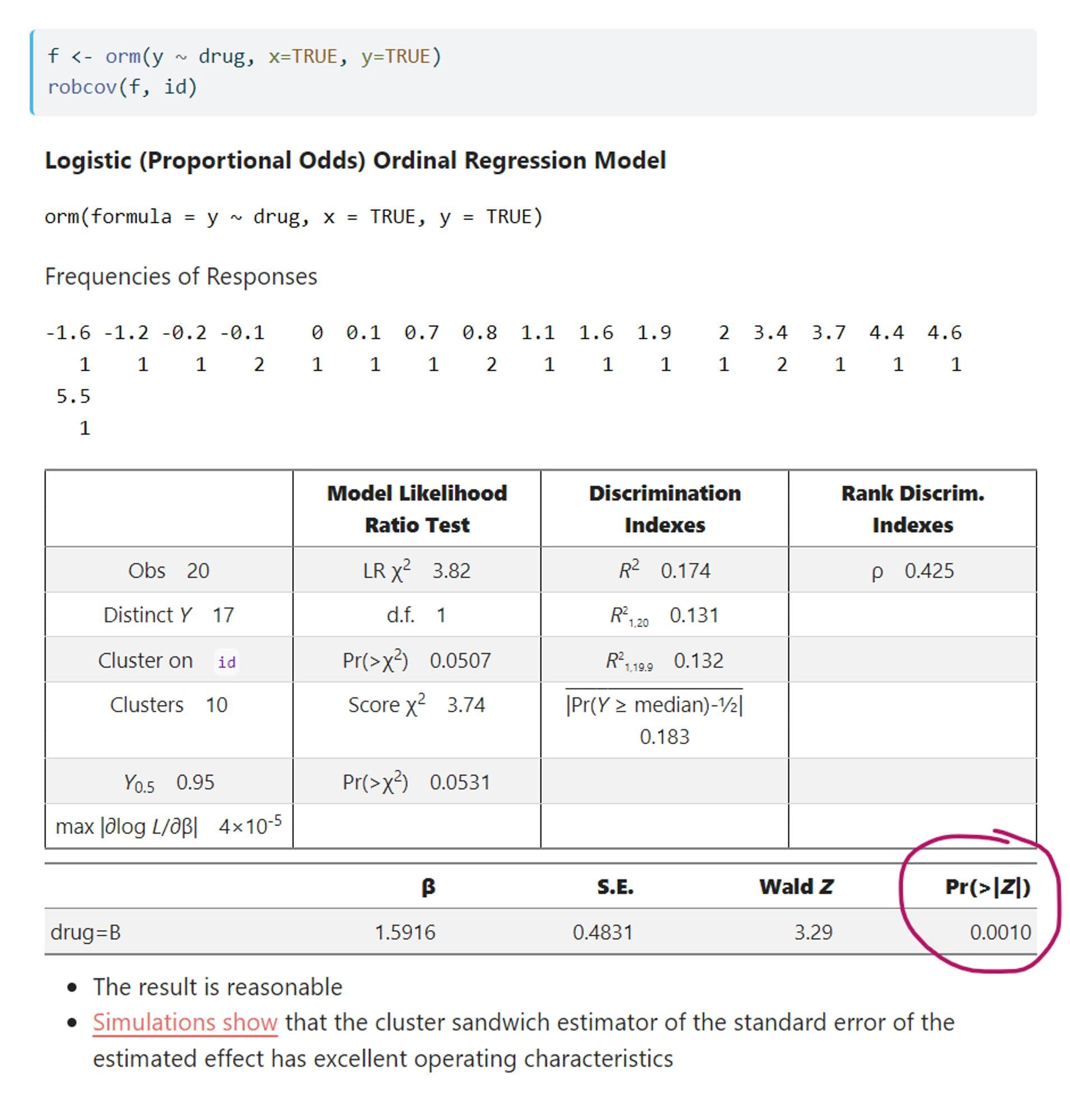
I’m trying to get the information needed to report a comparison of paired ordinal values. I followed the steps at the very end of section 7.9 here:

image

However, I can’t figure out how the print() function is calculating those values. Specifically, I’m trying to get the values needed to fill in these blanks:
X²(___) = ___, p = ___
(I’m not asking for help with the formatting. I just need help getting these values programmatically.)

For the p-value, I’m missing at least one step. And I can’t figure out the other parameters. Here is the book’s example:

f <- orm(y ~ drug, x=TRUE, y=TRUE)
model = robcov(f, id)

df = **what goes here???**
beta = model$coefficients
se = sqrt(diag(model$var))
Z = beta/se
p = 2 * (1 - pt(abs(Z), df))

Thank you,
Steve

Print model$stats and you’ll see the name of the element containing the number of non-intercepts, i.e., the d.f. for the likelihood ratio \chi^2. But we can’t use the LR \chi^2 itself if there was any clustering done.

Thank you @f2harrell. The content of model$stats is below. If the likelihood ratio X^2 can’t be used because clustering was done, what values should be reported? In other words, if I do this the wrong way and treat the ordinal responses as numeric in an ANOVA, I’d get F(, )=, p=. What do I replace that with, and how would I get those values?

> as.list(model$stats)
$Obs
[1] 71077

$`Distinct Y`
[1] 7

$`Median Y`
[1] 4

$`Max Deriv`
[1] 6.653846e-07

$`Model L.R.`
[1] 38804.36

$d.f.
[1] 1

$P
[1] 0

$Score
[1] 36755.55

$`Score P`
[1] 0

$rho
[1] 0.6744954

$R2
[1] 0.4335466

$`R2(71077)`
[1] 0.4207078

$`R2(1,71077)`
[1] 0.4206996

$`R2(67465.1)`
[1] 0.4373949

$`R2(1,67465.1)`
[1] 0.4373865

$g
[1] 1.521794

$gr
[1] 4.580435

$pdm
[1] 0.2886286

What you need is model$stats['d.f.'] but more coef(model) combined with vcov(model) to get sandwich-based Wald statistics. Usually better: anova(model) gives you a matrix of statistics. Pull off the needed row.

Hi,
I get this error when running plot(anova()) function
Error in dc(w, xlab = xlab, pch = pch, auxtitle = auxtitle, auxdata = auxdata, : labels not defined

I need to get the plot of variable importance of a cph()object obtaind from a database that has been transformed by sPCAgrid().
sparsePCA_trans_splines is a PcaPP (sPCAgrid()) object
coeff_numbers are specific coefficients I need to subset for the model

This is the code:

sparsePCAdataset ← sparsePCA_trans_splines$scores[,coeff_numbers]
colnames(sparsePCAdataset) ← c(“C3”,“C4”,“C7”,“C11”,“C13”,“C15”,“C16”,“C17”,“C18”,“C20”,“C21”,“C23”,“C24”,“C26”,“C28”,“C31”,“C34”,“C39”,“C40”,“C41”)
cox_cph_sparse_trans_splines ← cph(Surv(g$MTBR, g$STATUS) ~ sparsePCAdataset, surv=TRUE, x=TRUE, y=TRUE)
plot(anova(cox_cph_sparse_trans_splines,test=‘LR’,vnames=‘names’))

Does anybody know what is the cause of this error and how can I fix it?

Thank you so much for your help

Break it down:

a <- anova(....)
plot(a)

See where the error occurs. After the error type traceback(). Minor point: try not to use $ in formulas.

Hi, already fixed. This works:

coeff_numbers <- as.numeric(gsub("[^0-9]", "", names(gs_sparse_trans_splines)))

sparsePCAdataset <- sparsePCA_trans_splines$scores[,coeff_numbers]

sparsePCAdataset <- as.data.frame(cbind(g$MTBR,g$STATUS,sparsePCAdataset))

colnames(sparsePCAdataset) <- c("MTBR","STATUS","C3","C4","C7","C11","C13","C15","C16","C17","C18","C20","C21","C23","C24","C26","C28","C31","C34","C39","C40","C41")

cph_sparse_trans_splines <- cph(Surv(MTBR, STATUS) ~ C3+C4+C7+C11+C13+C15+C16+C17+C18+C20+C21+C23+C24+C26+C28+C31+C34+C39+C40+C41,data = sparsePCAdataset, surv=TRUE, x=TRUE, y=TRUE)

I had created a new dataset including the columns of status and time (thus avoiding $ reference to a different dataset where time and status data were available), then specified column names.

After, and this is what I think it was the problem: I had specified all the covariates of the model and included the term data = sparsePCAdataset. In the other case I just ran the model this way cph(Surv(g$MTBR, g$STATUS) ~ sparsePCAdataset, surv=TRUE, x=TRUE, y=TRUE)

Thank you for your help

1 Like

Hi,

I created a nomogram for a proportional odds logistic regression with 3 groups.

I modified the example code from this paper: DOI: 10.21037/atm.2017.04.01

#Samplecode

n <- 1000 # sample size 
set.seed(88) # set seed for replication 
age<- rnorm(n, 65, 11) 
lac<- round(abs(rnorm(n, 3, 1)),1) 
sex<- factor(sample(1:2,n,prob=c(0.6,0.4),TRUE), labels=c('male','female'))
shock<-factor(sample(1:4,n,prob=c(0.3,0.3,0.25,0.15), TRUE),
labels=c('no','mild','moderate','severe'))
z<- 0.2*age + 3*lac* as.numeric(sex)+ 5*as.numeric(shock) -rnorm(n,36,15) # linear combination with a bias
y <- ifelse(runif(n) <= plogis(z), 1, 0)

Y <- ifelse(y==0, 0, sample(1:3, length(y), TRUE)) 
data <- data.frame(age=age,lac=lac,sex=sex,shock=shock,y=y,Y=Y) 
var.labels = c(age="Age in Years", lac="lactate", sex="Sex of the participant", shock="shock", y="outcome",Y="ordinal")
label(data) = lapply(names(var.labels), function(x) label(data[,x]) = var.labels[x])


#Binary outcome
ddist <- datadist(data) 
options(datadist='ddist') 
mod.bi<-lrm(y~shock+lac*sex+age,data) 
nom.bi <- nomogram(mod.bi, lp.at=seq(-3,4,by=0.5), fun=function(x)1/(1+exp(-x)), fun.at=c(.001,.01,.05,seq(.1,.9,by=.1),.95,.99,.999), funlabel="Risk of Death", conf.int=c(0.1,0.7), abbrev=TRUE, minlength=1,lp=F)

plot(nom.bi,lplabel="Linear Predictor", fun.side=c(3,3,1,1,3,1,3,1,1,1,1,1,3), col.conf=c('red','green'), conf.space=c(0.1,0.5), label.every=3, col.grid = gray(c(0.8, 0.95)), which="shock")
legend.nomabbrev(nom.bi, which='shock', x=.5, y=.5)


# Ordinal outcome
mod.ord <- lrm(Y ~ age+rcs(lac,4)*sex)
mod.ord
fun2 <- function(x) plogis(x-mod.ord$coef[1]+mod.ord$coef[2])
fun3 <- function(x) plogis(x-mod.ord$coef[1]+mod.ord$coef[3])
f <- Newlabels(mod.ord, c(age='Age in Years')) 
f
nom.ord <- nomogram(f, fun=list('Prob Y>=1'=plogis, 'Prob Y>=2'=fun2, 'Prob Y=3'=fun3), lp=F, fun.at=c(.01,.05,seq(.1,.9,by=.1),.95,.99)) 
plot(nom.ord, lmgp=.2, cex.axis=.6)

How do I use the Mean function to add “the predicted mean Y from the PO model” (RMS, p. 319) to the code above?

@f2harrell. I reopen this thread as I have a very similar question
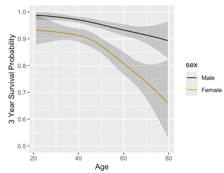
I am currently analyzing an interaction of a continuous and categorical variables in a survival model (age*treatment). I have seen the examples above and also in RMS ch 20. I think plotting both HR (ggplot.Predict (model, age, treatment, fun=exp)) and X-time survival probability stratified on treatment (ggplot.Predict (model, age, treatment, time=X) is very helpful (as below) and illustrative. Also plotting the HR in the range of the continuous variables using contrast.rms as explained in the example looks very good. I would like to ask 2 questions:

  1. Is there any correction for multiplicity? Is it needed?
  2. Is it possible to do contrast for the X-time (i.e: 2-year) survival probabilities between treatment A and B? In addition to plotting the HR as a relative measure of effect), it would be useful to provide a contrasts of an absolute measure of effect…

image

Very few analysts correct for multiplicity in these types of analyses but we all should. The contrast function has an option to easily do that through simultaneous contrast coverage.

Predict has a time argument to get 2-year estimates but contrast doesn’t.

1 Like

Hi Frank,

I am also facing this same issue. Do you know if there is a workaround?

Thank you!

There’s no automatic workaround but the solution is very programmable. At worst you can evaluate the difference inside a bootstrap loop to get a confidence interval.

Hi Frank, thanks for the quick reply.

I am sorry, but I didn’t understand your proposed solution.
Just to make sure we are on the same topic, my issue is not being able to have a lrm object with offset and no intercept nor covariates in the model.