Please pardon my ignorance. This question is based on my lack of understanding of how spline works.
I am working with chemicals data that have varying concentration with time. Lets assume this scenario, where during summer months when people drink a lot of water , it is hard to detect some these chemicals in their urine sample compared to winter or other seasons.
Instead of discretizing time and including time as an interaction term, I am interested in using a spline approach.
The fact that I cannot interpret the individual coefficients from spline model after modeling chemicals data as a function of spline is confusing to me. Is the utility restricted to visualizing the varying chemical concentration with respect to time using 2d plots (time on x axis) ? Any suggestions or advice on how to interpret output from spline model is much appreciated. Thanks.
Splines, not matter which basis functions you use (B-splines, natural splines, restricted cubic splines, …) are not intended to provide interpretable individual coefficients. They are intended to fit the relationship between X and Y so as to be able to adjust for this effect and to make predictions. Splines are interpreted graphically. During interpretation the whole spline function is used, not just pieces of it.
Please, is there a way to label cases on the residuals plots (fitted vs resid & qqnorm plots)?
I’ve used “i<-resid(f, ‘influence.measures’)” and “summary(i)” to produce hat and Cooks d values for all observations, but how do I identify the observations corresponding to the highest hat and Cooks d values obtained?
How relevant are these influence measures for a ols model using rcs?
The reason I’m asking is because there are probably a few observations in my dataset that are overly influencing my model and perhaps masking associations between predictors and the response. I want to indentify these cases/observations and then re-test the model without them to see what happens. Does that sound a reasonable approach?
The rms package which.influence package prints which observation numbers are overly influential, and it is comprehensive in the sense of looking for influence on any coefficient involving a predictor. This is especially useful when using regression splines.
Is it correct to look at influential cases only for the predictor(s) of interest, or should one look at influential cases for all predictors? For example, I’m mainly interested in testing the association between FM and the response variable. Thus, if I re-test the model only without cases 72, 92, 103, 130, and 144, would that be a sensible approach? Although there is some overlap among the predictors in terms of influential cases (e.g., cases 103 and 144 are influential for all predictors), if I take all influential cases into account (for all predictors) I would end up excluding a larger number of cases from the analysis when re-testing the model.
How do I know whether the influence of these cases is in one direction or the other? For example, are they following the relationship between FM and the response variable suggested by the fitted curve (partial effects plot) or they are going in the opposite direction of this relationship, and therefore masking a significant assoaciation (anova) between FM and the response variable?
I suppose the number on the column “Count” (which is produced by “show.influence”) is the number of betas that are influenced by the removal of that case, and the asterisks indicate the predictor(s) whose beta(s) are influenced. If that is correct, are the cases with the highest “Count” the most influential ones?
Another quick question: On the ANOVA table, for a predictor with 2df (3 knots), I have the results of the 2df test of association and of the 1df (nonlinear) test of association. What is the interpretation, in terms of the association between predictor and response, if only the 1df (nonlinear) test is statistically significant?
You’re probably right about Count; check the help file. Regarding the other question please study the notes or text on this chapter. It is not appropriate to look very hard at individual coefficients but look at the confidence bands overall and at the test of association with multiple degrees of freedom (tests flatness of overall association).
What I understand from chapter 2 of RMS is that we should first look at the multiple degree of freedom test of association from the anova before interpreting the partial effect plot. If this test is significant (meaning that X is associated with Y, or the curve is not flat), then we can “trust” on the curve we see (and then perhaps we can also look at the nonlinear test of association of X from the anova?). But I’m struggling to get my head around the following situations:
The predictor of interest has 2df (3 knots). The 2df test of association is nonsignificant, but the 1df (nonlinear) test of association is significant. Should we ignore the latter and conclude that there’s no association (i.e., the curve is flat)?
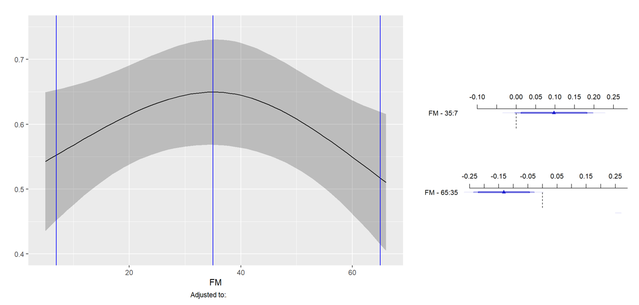
The 2df (overall) and the 1df (nonlinear) test of association are both significant and the curve has an inverted U shape. However, when computing partial effects using summary(), the effect of changing X from the .05 quantile (X=7) to the apex of the curve (X=35) is nonsignificant, but the effect of changing X from the apex to the .95 quantile (X=65) is significant (please see attached image). My interpretation is that this is simply a matter of power (insufficient observations on the first half of the curve), since the CI is almost entirely to the right of the summary() plot. Is this interpretation correct?
The default cutoff for detecting overly influential cases is dfbeta > 0.2. The example given on ?which.influence is a cutoff of 0.55. On what basis should we define this cutoff? Defining higher values is likely to identify fewer overly influential cases, and therefore cause less bias to the model when such cases are removed and the model is refitted. Correct?
It’s not that you can fully trust it (confidence bands are better for that) but that you have more license for interpreting the curve if you have evidence against non-flatness. Tests of nonlinearity should not be routinely done except to impress your boss that complexity exists so that SPSS should not replace statisticians.
Since you allowed for nonlinearity and specified that 2 parameters are used for the predictor you need to use only the 2 d.f. test. And “insignificant” results do not prove the null. You can just say that there is little evidence against the supposition of flatness.
This is an example where I regret writing the summary.rms function. It should ony be used for monotonic relationships (and sometimes I think it should only be used for known linear relationships).
All cutoffs are arbitrary and create game-playing. I don’t take influence statistics too seriously but use them as an opportunity to rethink pre-transformations to make the model more robust. For example heavy-right-tailed variables such as white blood count are best cube rooted before analysis.
Ok, I’m a little confused now. Are you saying that summary.rms should ideally only be used with categorical predictors and for linear relationships between X and Y?
On different topics now…
If I want to get robust tests that are not affected by, e.g., non-constant variance and/or non-normality of the residuals, can I use the bootcov.rms function? If yes, should I simply apply this function to the fit object and then use this new object, for instance, in the anova.rms to get robust tests of association? And then also use it in ggplot(Predict()) to get the ‘robust’ curves?
Finally, for dealing with outliers in my response variable, if I use quantile regression (Rq.rms), is the interpretation of the model the same as for ols.rms in terms of tests of assoaciation (anova.rms) and partial effects plots? Are there any peculiarities in Rq?
Robust variance estimates may be the correct estimates of the wrong quantity. They can’t fundamentally fix a misspecified model or one in which Y should have been transformed first.
Yes for the most part. Quantile regression requires larger sample sizes due to inefficiency.
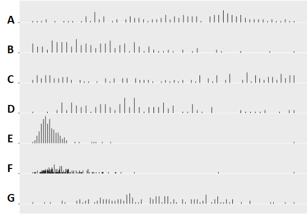
I have these continuous variables (see image attached). D to G are response variables. I have 4 ols regression models, one for each response. C is my main predictor of interest. I want to test the association between C and each of the response variables, separately in each model. A and B are adjustment variables. I also have categorical variables (e.g., sex) as adjustment variables. For example, in a given model I have:
F ~ rcs(A, 3) + rcs(B, 3) + rcs(C, 3) + SEX
I have transformed some of these continuous variables in different ways and then fitted the model above for each of the different transformations. For example, I have fitted the model above in 4 different scenarions:
no transformation
with a cube root transformation of B and F
curtailing outliers in B and F (outlier scores were replaced by the highest value just below them)
curtailing outliers in B and F (as above) and then performing a square root transformation of B and F scores
The problem now is that I don´t know which of the models above (1-4) I should choose for looking into the associaton of interest (between F and C). What should guide this decision? Residuals (in terms of their normality and constant variance)? Adjusted R^2? Likelihood Ratio Test?
bootcov does not necessarily apply here. You are not succeeding in maximally prespecifying the model. Spend much more time on the model formulation and much less time on model comparisons. For independent variables that are very skewed see if cube root yields a symmetric distribution. This may do away with the need for curtailment. For dependent variables consider semiparametric models which are Y-transformation invariant.
This is a Chapter 4 question and not a Chapter 2 question.
Ok, thanks.
Once I have pre-transformed and pre-specified the model, if my residuals (residuals vs fitted and normal qq plot) indicate non-constant variance and/or non-normality, does bootcov address the problem?
For example, using b<-bootcov(fit) and then anova(b)? Since my focus is on the multiple degree of freedom test of association.
bootcov and robcov help you in getting more accurate standard errors. But these can easily be the right standard errors on the wrong quantities if the model is not correct.
You don’t. You use loads of subject matter expertise to formulate the model and make it as flexible as the sample size allows. If there are 2 competing models we can do a pretty good job judging which one better fits.
When you make the model apriori as good as it can be within sample size limitations you have to ask what’s the alternative, because an alternative model can have different, worse, problems and can overfit. For example relaxing model assumptions can sometimes result in higher mean squared errors of prediction. Again, this is a Chapter 4 question.
Not sure whether this is the right place for this question. Apologies if not, but I never know for sure where to post my questions.
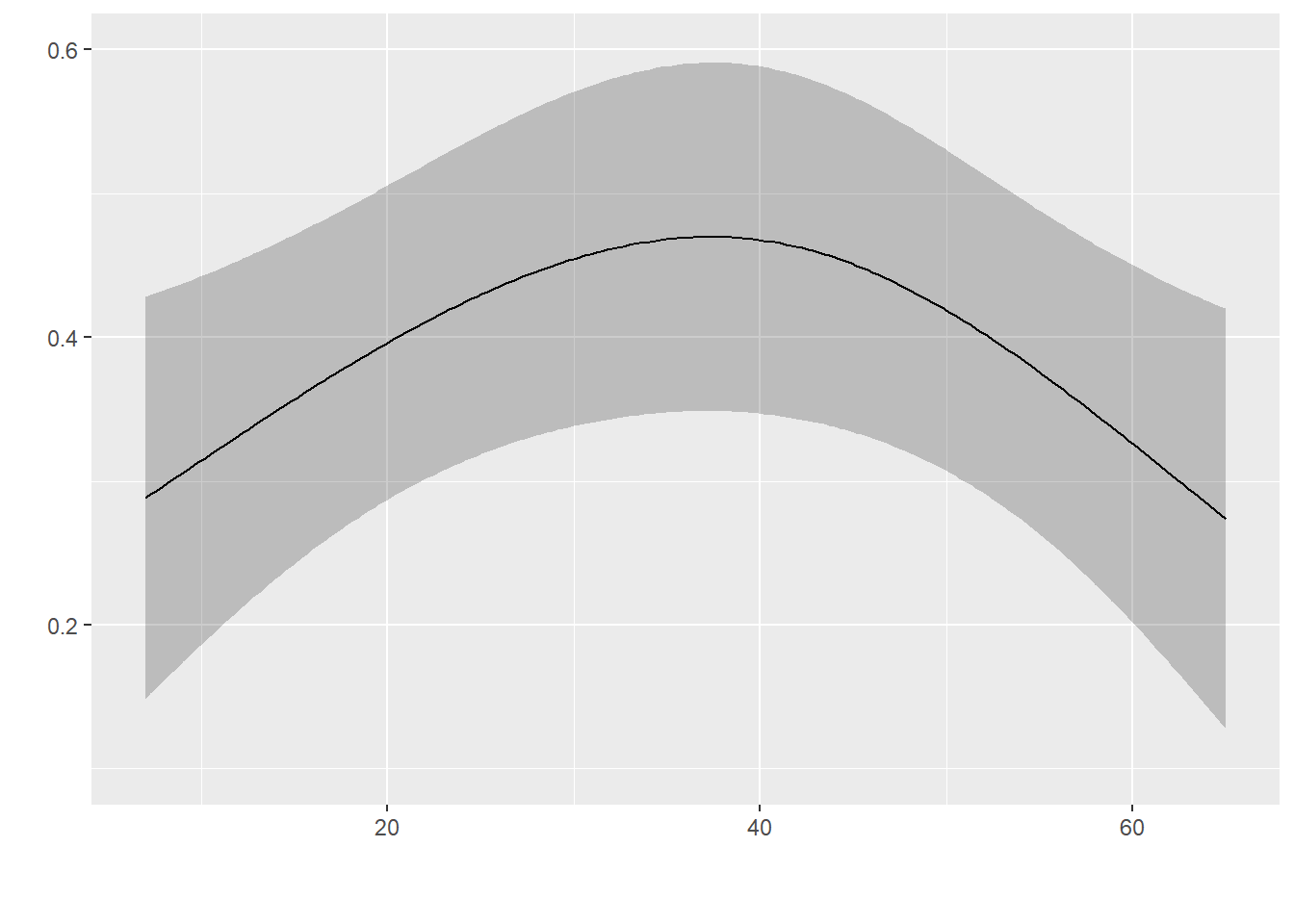
I have used bootcov to get robust estimates of association between my predictor of interest and the response variable. I first created my fit object (f), using rcs and adjustment covariates, and then used bootcov (b<-bootcov(f, B=1000)). Then I used the anova(b) to look at the multiple df test of association, and then ggplot(Predict(b)) to look at the partial effect plot. My question is:
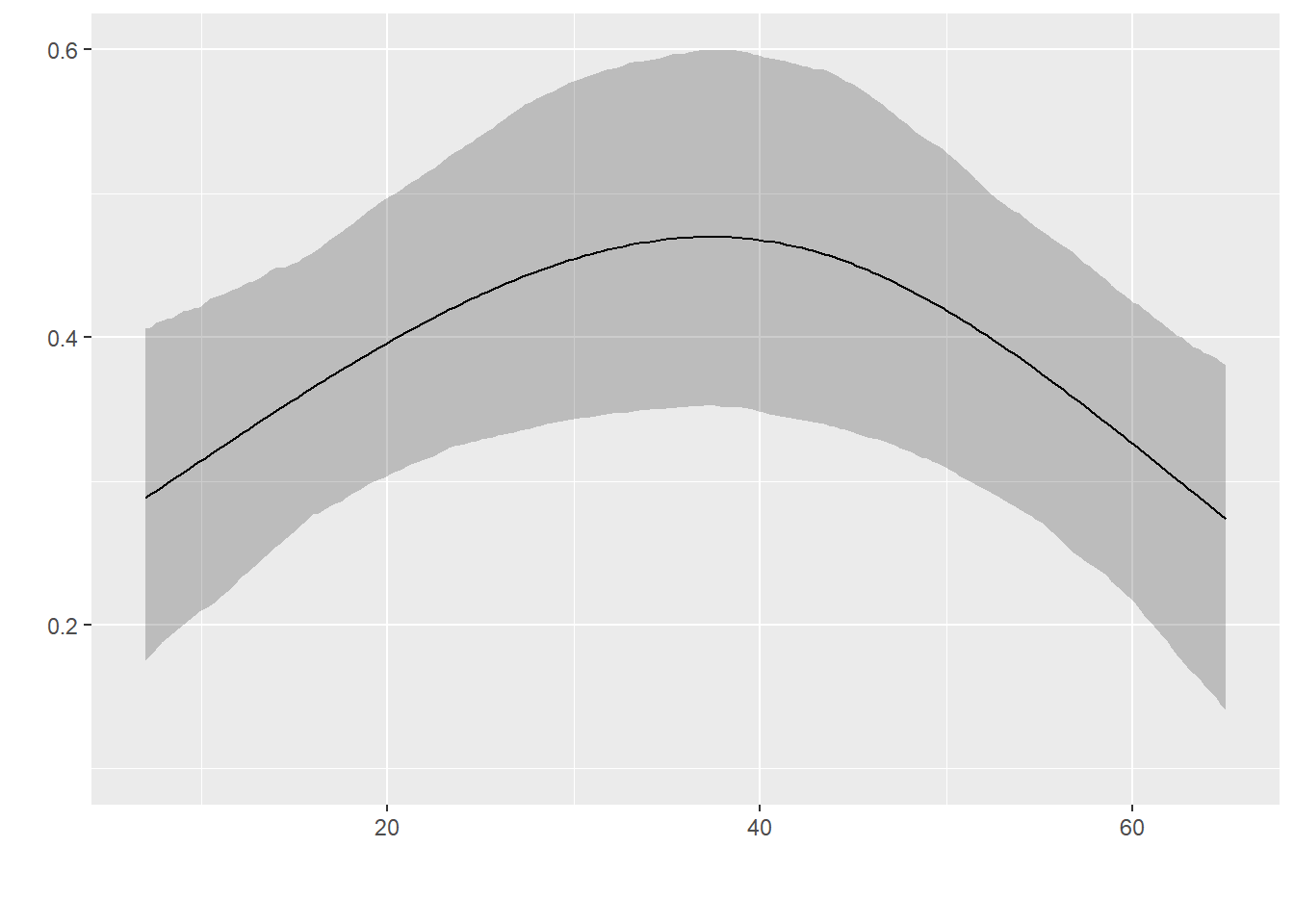
Why is the confidence band on this partial effect plot all wrinkled (see picture)? The confidence band from the partial effect plot produced without applying bootcov to the fit object is much smoother (see other picture). This is probably a silly question! Anyway…
There are two main types of bootstrap confidence intervals. First, you can use the bootstrap covariance matrix estimate to get Wald confidence intervals. These will be smooth. Second, you can use the bootstrap to get nonparametric percentile confidence intervals which are probability what was used here. The intervals are computed by getting quantiles separately at each X, and these will jitter around a bit.