OK, thank you!
But are there any downsides in doing what I have done (using the nonparametric percentile confidence intervals)? Are these CIs more robust to deviations of regresssion assumptions (normality and constant variance of residuals) than the Wald CIs?
What are the main uses of each of these 2 types of bootstrap CIs? Put another way, would I get different results from the anova and partial effect plot had I used the Wald CI?
It varies. In general I’m disappointed witih bootstrap percentile intervals. Best intervals use profile likelihood, but that’s more trouble.
Can I find more information about this subject (and more details on the bootcov function) on the RMS book or course notes?
Dear @f2harrell,
Please, I need some help.
When I run the anova on a bootcov fit object using R Markdown, I get a specific set of p-values for the tests of association. However, when I knit my results to html, the p-values from this anova change, as if another bootstrap was performed while knitting the outputs. Do you know why and how to fix this? Thank you!
Run set.seed(some integer value) before running a bootstrap or cross validation function. Do ?set.seed for details.
1 Like
Hi Frank, there is a predictor X1 that is highly correlated with the mediator variable M, in theory and according to experts X1&M are highly correlated. However in reality due to measurement error in X1 I am unable to include this predictor in my analysis. What are the implications of excluding X1 when in theory it is correlated with M ?
My guess is that excluding X1 will not hurt the coefficient estimates of variable M but this will reduce the SE of M and make the CI of M smaller. Is my assumption correct ? Please advise. Thanks.
1 Like
I wish I had experience with that. @Drew_Levy ?
1 Like
Hi Sudhi; The first thing to be concerned about is clarity about what the research question actually is—what is the specific scientific proposition you are trying to pose and evaluate. Substituting terms in a model without being clear about the subject matter implications for inference is what ought to be resolved initially.
Have you articulated what the particular estimand is that you are seeking (e.g., total effect or direct causal effect of X1 on Y)? Have you drawn a DAG to support your thinking? That might be the first step to get a credible analysis. If you are new to that process, an accessible, informative, and even fun introduction might be Statistical Rethinking 2023 - Lecture 5; and, maybe especially Statistical Rethinking 2023 - Lecture 04 for your particular query.
It really depends on the causal relationship posited between X1 and M: “correlated” is an ambiguous term and assignation. Without more background/detail/understanding, it would seem that by omitting X1 you are making X1 an unobservable parent of M. If there are not backdoor paths between X1 and Y then evaluating the relationship M → Y might be straightforward. But this changes/distorts the actual research question and requires strong assumptions about the causal processes for Y.
A good intro for your purposes may be Causal Directed Acyclic Graphs, JAMA 2022.
I hope all this is closer to useful information than aggravation.
drew
2 Likes
Thanks Drew. I am trying to estimate the causal effect of X1 on Y. I have a DAG but that keeps on changing, you made several good suggestions here. I will work on those. Thanks again.
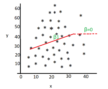
@f2harrell , Hi Frank somewhere in your lecture, either 2 or 3 I dont remember exactly where, you mentioned you were breaking the linear regression line into two segments and forcing the right side to be horizontal so that the beta for this portion is zero.
Can you please point me to an example how this is implemented ? Thanks.
I discuss that in Chapter 4 under the topic of overly influential observations but don’t actually show it. Here is what code looks like:
f <- lrm(y ~ sex + pol(age, 2) + rcs(pmin(x, 30), 4))
Or you can use gTrans if you need more exotic models such as one allowing for a discontinuity at 30.
1 Like
Thanks Frank, so this means the pmin function will force x >30 to be 30.but y values will be different. This will not bias the results because the beta_hat = 0 for x>30
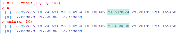
This treats x > 30 as 30 so makes any predicted Y at x > 30 to be the same predicted value had x been 30. It is not quite right to say that \hat{\beta} = 0 for x > 30. It’s better to say that \hat{\beta} applies to x \leq 30, i.e., it is the slope for x \leq 30.
1 Like
Is there a way to fix the value of one predictor when specifying a nomogram (that is, instead of including an axis for it)?
Try specifying axis limits for that variable that only has one point. Otherwise we’ll need to come up with another way.
1 Like
Frank is there a difference between the Predict function from rms library and the regular predict function ? Whats the advantage in using Predict function from rms compared to the old vanilla predict function.
Besides the minor point of handling restricted interaction terms (%ia%), Predict allows you to omit any and all data settings for obtaining predictions, and reasonable defaults will be used. These defaults come from datadist. And Predict allows time= to make it easy to get survival probability estimates.
When you are varying only one or two variables, and especially when these don’t interact with other variables, you can omit the values of the other variables when using Predict.
Predict produces a data frame ready for plotting with rms functions plot, plotp, ggplot or by using the full ggplot2 package.
1 Like
Thanks Frank, I think , when I use to fortify function and export the dataset from Predict function it gives me an option to see what was generated and how. Also allows me to customize few things. So great.
Just type str(Predict(...)) and ?Predict and you’ll see all that.
1 Like