Hello Prof Harrell,
Thank you so much for the RMS class.
My team is trying to estimate GFR for cirrhotic patients. Expert knowledge indicated using as predictors Age, Sex, Albumin, BUN, and CR and they indicated a possibility to pre-specify an interaction between Sex and Cr.
Physicians also suggested exploring if an interaction exist between Alb and Sex or between BUN and Sex based on data. As we learned at the RMS course, we should avoid exploring interactions that are not pre-defined.
Inker at all (2021) (https://www.nejm.org/doi/full/10.1056/NEJMoa2102953) estimated a new GFR equation (removing race) using a least squares linear regression relating log transformed measured GFR to log-transformed Cr, age, sex with two slope linear splines for log-transformed creatinine, with a knot at 0.7 mg/dl for women and at 0.9 mg/dl for men.
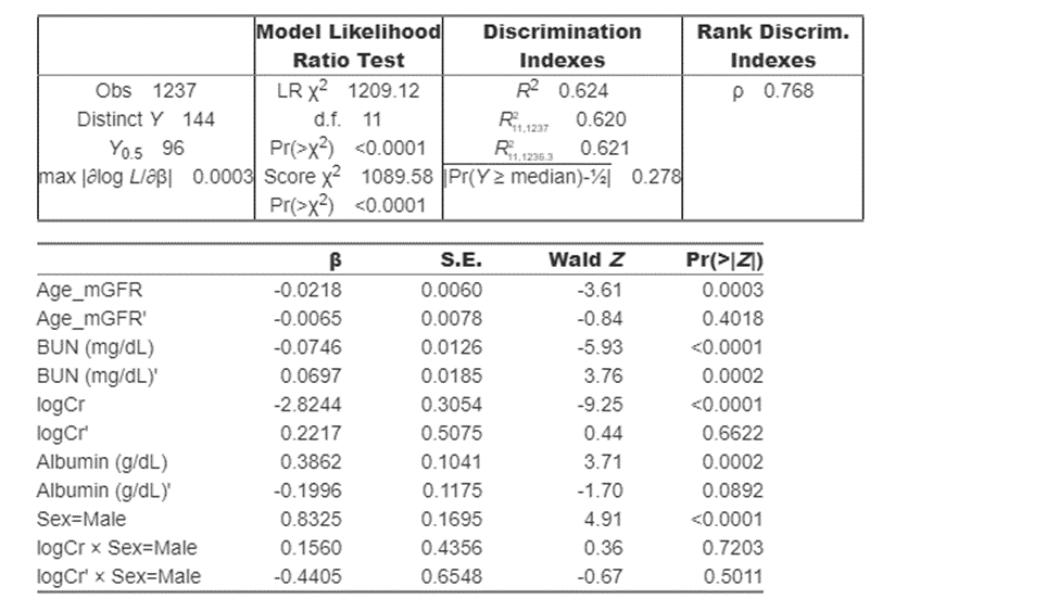
Estimated GFR equations don’t work well for cirrhotic patients. They perform very poorly for low value of GFR. In our specific case of cirrhotic patients, the goal is to improve the estimations at the extreme values, (low GFR values). About 5% of our sample has GFR measures ≤30. The total sample size is 1237. The dependent variable is skewed and presents a lot of ties. For these reasons, I am considering a cumulative probability ordinal model with Y continuous.
(Dr. Harrel, I was in your class when you mentioned your experience with the estimated GFR model)
Here is my first attempt. I am finding that the interaction between CR and Sex is not significant. However, since it was pre-specified, I could leave it in the model.
Physicians found it strange that the interaction between Sex and Cr is not significant in the and asked if we can come up with a cut off for the creatinine different for male and female, like what was found in the Inker’s equation.
My questions. Is it ok to leave the interaction in the model? Should I try to consider different slopes for male and female as the physicians suggest or just leaving the interaction in the moder should be, ok? Is this the right way to improve the prediction at the lower tail? Or maybe a quantile regression if ties are not so much a problem. Here is my starting point. Thanks
Hello Prof. @f2harrell,
When I run
Predict(bootcov(f), x, boot.type = 'bca')
I get the following:
Warning: ‘.Random.seed[1]’ is not a valid Normal type, so ignored
The warning keeps repeating hundreds of times until Predict() is completed.
The function seems to work fine, but how to get around this warning?
Thank you!
@arthur_albuquerque, do you know?
It is a tough question to know whether or not to leave the interaction in the model. I’m tempted to leave it.
Linear splines have elbows that don’t match physiology so I’m a bit converned about their use.
We need a measure of lean muscle mass instead of a binary sex variable for this purpose.
Put 'bca' in quotes.
Hello everyone!
I have a spline term in a Cox model with rcs(). What plots could I use to see how well the spline fits the “data”? I’m not sure what kind of data the spline should fit.
Thanks in advance for the answers.
The deeper question is whether having a better fit is worth it, i.e., you need to consider the variance-bias tradeoff. Thinking more shallow, you can compare a spline fit with a nonparametric smoother as a feel-good check, especially if there are no other covariates.
We need to think more about the impact of lack of fit and of fitting more parameters, rather than just thinking about goodness of fit. For more see this.
A higher p-value for non-linearity indicates that the restricted cubic spline is closer to a straight line; however, sometimes the graph differs from the p-value for non-linearity. For example, in the case of C, I perceive it as not being a straight line, yet its p-value for non-linearity is 0.44.
Also, sometimes the p-value is less than 0.05, but it appears to be a straight line.
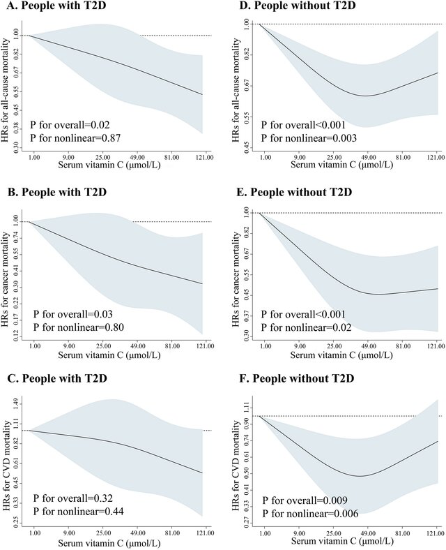
As for me, I do not trust the p-value, so I prefer to decide the linearity based on the graphics. Different sample size may explain the inconsistent. In the case of C, I don’t think it represents a straight line.
I would like to know your insights when the restricted cubic spline and p-value for non-linearity display contrasting results regarding linearity.
You are right to place little trust in p-values. Here a large p-value means that you did not assemble enough evidence to contradict a supposition of linearity. This is far from saying that there is evidence of linearity, especially since large p-values can result from small sample sizes. The confidence bands tall you more.
It’s better to assume that everything is nonlinear and then to just quantify how much of the estimated relationship is nonlinear. So perhaps more valuable quantities to put on the plots would be partial pseudo R^2 for the likelihood ratio chunk test of association for each variable, and what proportion of the likelihood ratio \chi^2 is due to estimated nonlinear effects. For more about R^2 see here.
Thank you very much for the clarification, professor harrell.
Assuming
My outcome(y) is a continuous variable, for example : Children’s IQ score.
I am fitting a simple linear model to predict y, and one of the term in my model is an interaction between , lead content, exposure(continuous y) and child sex(1Male, 2Female), the reference level is 1Male.
If these are my estimates from fitting this model
Terms                     Estimates   Std.Error      p.value
Intercept                 2012.12       1234.56       0.1234
Lead(Exposure)              -6.5432       4.321       0.1122
Sex(Female)                -30.98        112.12       0.0005
Lead(Exposure)*Sex(Female)  21.12          4.321      0.013
How do I correctly interpret the estimates from the interaction term., including their CIs (Confidence intervals). I have some ideas about this but I have been looking at data far too long and became a bit rusty on few other things. Please pardon my ignorance. Thanks
It’s hard to explain the interpretation of the estimate for the interaction term without first looking at the the other estimates. As the reference group for sex is set to “Male” and since you haven’t centered the lead exposure the interpretation of the coefficients are as follows:
-
Intercept: The estimated IQ-score for a male with a lead exposure of 0. I.e. the estimated IQ-score for such a man is 2012.1!! This is hardly realistic. If you want an estimate that makes more sense you could mean-center the lead exposure variable and re-run the analysis using this variable instead of the actual lead exposure. This will have the effect of changing the interpretation of the new intercept to be the estimated IQ-score for a man with an average/mean exposure to lead.
-
Sex(Female): The estimated difference in IQ-score between a male and a female that both have a lead exposure of zero. I.e., the estimated IQ-score is 31.0 points lower for the woman than the man. If, as suggested above, you mean-center the lead exposure and rerun the analysis, the interpretation of the new estimate becomes the difference between a man and a woman that both have an average/mean lead exposure.
-
Lead(Exposure): The slope of the regression line for men. I.e., it is the difference in IQ-score between two men where one has a lead exposure that is 1 unit higher than the other. The person with the higher lead exposure will have an estimated IQ-score that is 6.5 points lower than the person with the lower lead exposure.
-
Lead(Exposure)*Sex(Female): The difference in slopes between the regression line for men and women. I.e. the slope of the regression line for women is 21.1 higher than the slope for men, which means that the slope for women is 14.6 (= -6.5 + 21.1). An approximate 95% 2-sided CI for the difference in slopes is given by 21.1 +/- 1.96 x 4.3 = [12.6 ; 29.4].
For how to correctly interpret the p-value and 95% CI I suggest you take a look at this thread: https://discourse.datamethods.org/t/language-for-communicating-frequentist-results-about-treatment-effects/934
Dear @f2harrell ,
after using a restricted cubic splines model in a manuscript, I was questioned why I did not implement smooth splines or LOESS, and that using 0.1, 0.5, 0.9 for the knots is ad-hoc.
I am arguing that
- RCS is better for inference for general audience
- it is general practice to place the knots there
- using three knots is based on the sample size I have
- it is easy to compare the models with linear ones via Likelihood-ratio test to derive p-values.
Can you recommend any further points or literature for this issue ?
Thanks a lot in advance!
I’d say that
- based on your effective sample size you wanted to spend two degrees of freedom (parameters) in estimating the extent and shape of association
- there was no subject matter to guide the specification of the shape of the relationship
- placing knots at quantiles as you did puts an equal sample size between any two knots, following the idea that you allow for shape changes where the data are rich enough to be able to estimate the relationship
- regression splines provide equations and simple inference (unlike smoothing splines)
- regression splines provide estimated curves that are usually in great agreement with estimates from nonparametric regression methods or smoothing splines
I am fitting a linear mixed effects model, the outcome is continuous and i have 5 covariates. One covariate is a discrete variable with 5 levels.
The model converges and I get meaningful estimates for all parameter , but a sub level in the discrete covariate(X5, level 4) has NA for standard error
factors           estimates      SE      statistic        df         p-value
Intercept       10.123           1.45    2.56            100.45  0.67
x1              0.4567           1.46   2.45             97.56   0.34
.
.
x5-level2      0.1234            1.23   3.45             96.12    0.12
x5-level3      0.1114            1.19   1.45             92.12    0.11
x5-level4      0.0223            NA    NA                NA       NA
I am wondering what could be the cause for NAs in just one sublevel of a factor variable.
Thanks.
What are the frequencies of all the levels of x5?
Hi Frank good question,
L1,L2…L5 are the levels in my covariate x5
A,B,C,D are the centers which is the random intercept in my model.
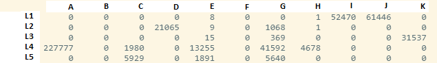
L3 is kind of a K thing so maybe that degree of collinearity between L3 and a random effect is a problem?
Thanks Frank that is in line with reality, some center strictly use one approach(levels of x5). So your suggestion makes sense.
Hi Frank you said in your lecture that AIC is useful for evaluating model complexity (linear vs non linear or interaction) what about Likelihood Ratio Test, is that not useful when comparing simple vs complex models ?
There are three approachs: LR test (F test in ordinary regression), AIC, and R^{2}_\text{adj}. LR is more compatible with R^{2}_\text{adj} but still different. They ask whether the bigger model is worth the extra parameters, in terms of statistical information. This is an in-sample assessment, i.e., they assess predictive discrimination for the current matrix of all predictor values. R^{2}_\text{adj} penalizes for p, the number of predictor parameters. AIC penalizes for 2p which contains an additional p penalty for asking about out-of-sample predictive discrimination. Minimizing AIC is an attempt to achieve the best log-likelihood in future samples when \hat{\beta} is frozen from the original sample.