This question is regarding centering, I have worked on studies where I was requested to center some continuous variables and in few other studies where we did not center the variables. Also if I remember correctly LASSO models requires centering continuous variables, what is the correct approach here ? when should we center the variables before analysis and when it is okay to ignore centering ? Thanks.
No methods I know of require centering predictors unless you are using very old linear algebra software in fitting. lasso depends only on careful scaling.
1 Like
Thanks Frank, may be this has more utility in interpretation ?
No, except possibly in interpreting interaction terms. But I don’t interpret them alone anyway.
1 Like
Dear prof. @f2harrell, I’m trying to reproduce the results which are obtained using the summary() function. Specifically, I want to manually estimate the standard error of the interquartile coefficient of a continuous variable included in a model fitted with cph.
I did understand how to do that starting from vcov(model) in order to get the variance associated with my predictor of interest.
My question is how to do that when the continuous variable is fitted using rcs(). In that case, vcov(model) generates a matrix in which every splines terms is included. Starting from this, how can I estimate the standard error of the continuous variable?
require(rms)
require(survival)
fit ← cph(Surv(dtime, death) ~ rcs(age, 4) , data = rotterdam, x = TRUE , y=TRUE)
vcov(fit)
Thanks
You’ll see in the code to summary.rms that there is a matrix product to compute the needed standard error after forming the difference in design matrices that leads to the effect of interest.
@f2harrell I had a look at the code but my understanding of linear algebra and R programming is not enough to grasp what is going on there.
Could you please elaborate more on this or suggest some source to study the general theory behind that?
Thanks
Since your goal is to compute the standard error manually and not use the functions I provided for this you can’t avoid looking under the hood.
Dear @f2harrell,
I have found the RMS book’s treatment of non-linearity particularly interesting, given that in my field, effects in regression are very often assumed to be linear (and I suspect are often not!).
One thing I am not clear on is how one should approach testing statistical significance of restricted cubic splines when residuals are non-normal, and the bootstraps produced by bootcov are themselves not normally distributed.
With linear effects, where a predictor is represented by a single coefficient, my usual approach when residuals are non-normal would be to apply a non-parametric bootstrap, and obtain BCa confidence intervals to account for any skew in the bootstraps of coefficients.
However, this approach to skew in the bootstrap isn’t available when a single predictor is represented by multiple coefficients (as is the case with restricted cubic splines). I know that the rms package helpfully has the bootcov command, and objects produced by bootcov can be examined with the anova command to get p-values from a bootstrap (and I believe bootcov uses non-parametric bootstrapping).
But when the bootstrap itself is non-normal, and should therefore be corrected by something like BCa, I’m not sure how I can assess the joint significance of a predictor. I could get BCa CIs of each individual coefficient, but as you explain in the book (and elsewhere online), interpreting these coefficients individually is difficult (or maybe impossible?)
Could you please explain how one should approach how to interpret statistical significance of restricted cubic splines when the bootstrap produced by bootcov is itself not normally distributed?
As a side note, the bootstrap distribution may only be a rough approximation to a sampling distribution, and judging the normality of a bootstrap distribution needs a bit more thought.
The traditional parametric frequentist approach to this problem just has too many problems. This is why I almost never use linear models any more, opting for frequentist or Bayesian ordinal semiparametric models as covered in later chapters of RMS. These don’t make distributional assumptions at any specific covariate setting.
1 Like
Hi Frank, Hope I am posting this question under the right thread. Please pardon my ignorance. I am trying to learn how to fit a model based on the 1st or 2nd derivatives of spline functions.
(rcs(pH, 3)
How do I take the second derivative of this spline function (rcs(pH, 3) and test this using simple linear model.
lm1 <- ols(residual_sugar ~ (rcs(pH, 3) + rcs(sulphates, 3))^2, data = mydata, x = TRUE, y = TRUE) print(lm1, coefs = FALSE)
Additionally, I would greatly appreciate any references to articles that have applied this methodology and provided interpretations of the results.
Thanks.
A new section in that chapter’s course notes shows how to fit a Bayesian model where it’s easy to put restrictions on the second derivative when representing that derivative as a double difference in predicted values over well-chosen values of x. You could use the contrast function to do something similar with a traditional frequentist model. This is not exactly evaluating a 2nd derivative but is approximating it with finite differences. To get at exact second derivatives would require more work, especially if x interacts with another variable. Start with the expression for the RCS in unrestricted form that has 2 redundant terms. The second derivative with respect to x is 6\sum_{i=1}^{k} \beta_{i+1}(x - t_{i})_{+}. See if that leads to anything useful.
![]() Also make use of the fact that the 2nd derivative is forced to be zero in an RCS when x \geq t_{k}.
Also make use of the fact that the 2nd derivative is forced to be zero in an RCS when x \geq t_{k}.
1 Like
Dear @f2harrell ,
I’m interested in probing an interaction between a restricted cubic spline and a grouping variable. In RMS terms, the model would be something like:
fit <- ols(y ~ rcs(x1, 5)*g + rcs(x2, 3)*g + rcs(x3, 3)*g)
Where x1 is my primary variable of interest, x2 and x3 are (less important) covariates (hence the difference in knots from x1), g is a grouping variable (5 data collection locations/groups), and total N = about 1500.
My primary interest is the question: does x1 relate to y, controlling for x2 and x3? Interactions with g are not of primary interest: I merely want to be rigorous, and allow for the theoretical possibility that these relationships I’m testing for might differ between data collection groups (which, due to the nature of this data collection, differ in age, country, socioeconomic status, etc).
I have a couple of questions:
Question 1. I’m used to terminology of “simple effects” and “simple slopes” when it comes to probing interactions in linear models. For example, if I had the model:
lin_fit <- lm(y ~ x*g)
If the interaction turned out significant, I’d look at the output of the emtrends command (from the emmeans R package), or alternatively run the model several times, changing the reference group of g each time, and look at the coefficient/p-value for x each time. I’d understand these effects as “simple effects”: the effect of x on y, separately for each level of g (as opposed to a “main effect”, which would be the effect of x on y, averaged over all levels of g).
Having looked through the datamethods forum, the RMS book, and the rms manual on CRAN, I haven’t seen any discussion of this idea of simple effects applied to restricted cubic splines. The examples in the RMS book and the rms manual suggest that your preferred method of testing interactions between restricted cubic splines and group variables is using contrasts, which can answer the question, how do two nominated groups’ curves (non-linear effects of x on y) differ at different levels of x?
I can see why that question is useful in many circumstances, but the question I want to ask answer is: within each group, is the wiggly relationship between x and y better than a flat line relationship with no gradient (to a statistically significant degree)? This is a different question to the one answered by the contrast method.
Is this something that can be tested? Sure, I could run each group as a separate regression and look at the effect of x on y within each group, but I understand some reviewers will want to know “is the interaction between group and effect of x on y statistically significant” before looking at the effects, within groups.
Question 2. When there are interactions included in a model, anova.rms() rolls the interaction term into the overall effect for each predictor, and doesn’t present the “main effect” by itself. For example, using some simulated data:
ols(formula = y ~ x * g)

 Factor                               d.f. Partial SS MS          F       P
 x  (Factor+Higher Order Factors)       3  88328.40   29442.80091 1252.32 <.0001
  All Interactions                      2  33450.47   16725.23479  711.39 <.0001
I’m used to thinking about main effects as being presented separately to interaction effects. Clearly what anova.rms() is doing is providing a “total effect” of x, which includes any of the higher order interactions, as well as the main effect.
Could you please explain the rationale for this? Is it possible to ask anova.rms for the main effect separated out from the interaction (as I expect reviewers will want to see the main effects presented separately to interaction effects). Alternatively, is there a reference I can show to a reviewer that justifies rolling the interaction into each main effect?
Many thanks!
(Note: I am not a statistician, merely an applied researcher. Please forgive my statistical ignorance if what I’m asking is extremely obvious. I’m here because I’m trying to improve my skillset!)
1 Like
Contrasts are always helpful. But in RMS I emphasize anova() in automatically doing meaningful chunk tests. It is impossible to uniquely define a separate main effect as this is coding/centering-dependent. Combined effects are coding/centering-independent and have perfect multiplicity adjustments. A combined effect tests a very meaningful thing and takes into account all the opportunities for something to have an effect. For example in a linear age x sex interaction the total effect of age is the effect for either sex, without assuming equal age slopes for males and females. The total effect for sex asks where sex has an effect for any age.
1 Like
Dear @f2harrell ,
Following our earlier conversation about probing interactions between restricted cubic splines and categorical variables, I had a thought I wanted to run by you:
My goal is to test a model examining the relationships between Y and several Xs that allows for the possibility that these Y on X relationships may be different at the different levels of categorical variable G. I’d fit a model like:
ols_model <- ols(Y ~ rcs(X1, 5)*G + rcs(X2, 5)*G)
If the G * X1 (Factor+Higher Order Factors) interaction is significant in the anova(ols_model) output, I’d like to ask: at what levels of G is the relationship between Y and X1 significant?
As best as my non-statistician brain can work out from reading the rms documentation, the rms::contrast function is helpful for answering the question, “is Y on X at G = 1 different to Y on X at G = 2”, but as best as I can tell it doesn’t allow me to answer the questions I’d like to ask (i.e., “is Y on X significantly different to 0 at G = 1? is Y on X different to 0 at G = 2?” etc).
It’s occurred to me I could emulate the logic of the emtrends function of the emmeans package (used to obtain tests of the linear relationship between X and Y, at each level of G) but with restricted cubic splines, by using the linearHypothesis function from the car package in conjunction with rms. That function allows one to specify a model, and several terms in that model that you’d like to compare to 0, and obtain an F test of the difference between the full and reduced models. I’d run the following:
lm_model <- lm(Y ~ rcs(X1, 5)*G + rcs(X2, 5)*G)
print(linearHypothesis(lm_model, c("rcs(X1, 5)X1", "rcs(X1, 5)X1'", "rcs(X1, 5)X1''", "rcs(X1, 5)X1'''")))
This would give me a chunk test that answers the question “are all of the RCS coefficients for X1 equal to 0”, which I think answers the question, is Y on X1 significant at the reference level of G? I’d then change the reference level for G using relevel(), rerun the model, and use linearHypothesis in the manner described, for each level of G. This would answer the question “is Y on X significant?” at each level of G. When testing these effects, I’d adjust alpha for multiple comparisons (.05/number of levels). And I could repeat the process for Y on X2 for each level of G.
That seems intuitive (although highly laborious) to my non-statistician brain. Would you say this is an acceptable approach to answering my question?
contrast (contrast.rms) does handle this. See its examples of double difference contrasts. But I would rather not think of this as a place for testing statistical ‘significance’ but rather a place for getting a partial effects plot with the continuous variable on the x-axis and separate curves for the interacting categorical variable. Estimation rather than hypothesis testing.
1 Like
Many thanks as always @f2harrell.
Regarding the plot method: I imagine such a partial plot would be obtained by running plot(Predict(model, X1, group = levels(dataframe$group), and I’d be looking not so much for non-overlapping CIs, but more how each line deviates from the others, and describing those deviations - is that correct?
Regarding the contrast.rms method (in case a reviewer asks): My apologies, I think I’m misunderstanding the contrast.rms examples. The only double difference contrast example (i.e., the one with 4 list() arguments) I see is the following:
f <- lrm(y ~ pol(age,2)*sex)
# Test for interaction between age and sex, duplicating anova
contrast(f,
     list(sex='female', age=30),
     list(sex='male', age=30),
     list(sex='female', age=c(40,50)),
     list(sex='male', age=c(40,50)),
     type='joint')
Which (as the comment says) represents the overall interaction of pol(age,2) and sex in model f. I don’t quite understand how to go from this code, to code that tests whether sex by age is significant (i.e., different to a null function) within females, and separately, if it’s significant within males.
My best attempt is as follows: If I were examining the relationship within females, for example, I think I should be comparing the predicted line of y ~ pol(age, 2) within females to a null function (i.e., a straight line, with gradient 0, with a y-intercept equal to the predicted y for females, averaged across all ages). Assuming I used ols and rcs, just to make it closer to my situation, I imagine it should look a little like this:
female_min_age <- min(dataframe$age[dataframe$sex == "female"])
female_max_age <- max(dataframe$age[dataframe$sex == "female"])
rcsmod <- ols(y ~ rcs(age, 3)*sex)
contrast(rcsmod,
     list(sex='female', age = seq(female_min_age, female_max_age),
     list(sex='female'),
     type = "joint")
Is that remotely correct?
ggplot instead of plot is a little nicer. And don’t include =levels(..) is this is automatically done for you.
Testing an age x sex interaction is only done when you combine males and females, so your interpretation is off.
The last part is not remotely correct. Go back to basics. For the double difference contrast you are interested in with 4 list()s. The only drawback of that is that since age is not assumed to be nonlinear, the results will depend on the 2 age values you select.
1 Like
I am curious about the differences between assuming a negative binomial distribution vs a truncated normal distribution, for my outcome variable(y) . Here’s the context:
An assessment test is administered , aiming to evaluate participants’ restlessness. The responses to these questions are aggregated, resulting in a continuous total score ranging from 0 to 150. Subsequently, this total score is transformed into a population-level t-score, with a presumed mean of 50 and standard deviation of 10. This t-score, is my outcome (y),
The distribution of this t-score, assumed to follow a normal distribution, is skewed, ranging from 27 to 100. A considerable number of participants exhibit lower scores, with fewer participants achieving higher scores. Lower scores are good, this means the participants are not restless.
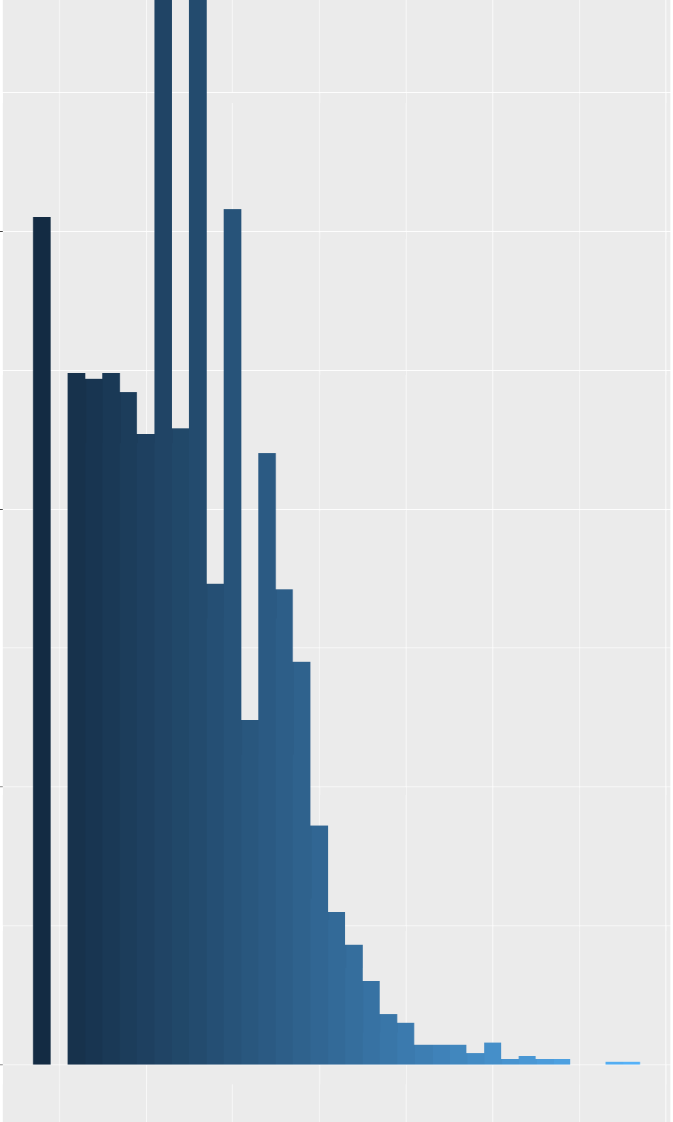
My question is what are the trade offs when I assume my outcome follows a truncated normal distribution versus a negative binomial distribution. This is a repeated measure data. There are 1000 participants and I have repeated observations (2 or 3) for 400 and only single measure for 600 participants. Your advice is greatly appreciated. Thanks in advance.
This should have been posted in the ordinal regression intro chapter or in chapter 4. The overall answer is that parametric models for continuous and count data assume too much, and the results are too sensitive to how you transform Y. That’s why I push semiparametric models so much.
1 Like