Got it, will do. Thank you Frank.
Dear @f2harrell, I’m trying to get a good understanding of what there is behind the equations currently used to estimate glomerular filtration rate. I’m currently focusing on the CKD-EPI creatinine 2021 where linear regression is used to model ln(GFR) according to ln(creatinine), age (on natural scale), and sex ( paper )
This is what the authors claim in the supplementary appendix
As we have previously described, CKD-EPI equations are modeled using least squares linear regression to relate log transformed measured GFR to log-transformed filtration markers, age, and sex with two slope splines for creatinine. The splines are two phase linear splines on the log scale. For creatinine, the knot is at 0.7 mg/dl for women and 0.9 mg/dl for men
This is how they report the equation in the general form (natural scale)

I have a simulated dataset with GFR, creatinine, sex, and age, and I’m trying to reproduce their model developing process to have a better understanding.
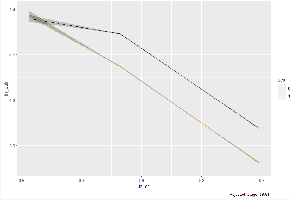
I use linear regression to model ln(GFR) with ln(cr), age (natural scale), and sex. ln(cr) is modelled as linear spline with one knot at ln(0.9) and ln(cr) X sex interaction is allowed.
# knot
k <- 0.9
ln_k <- log(k)

fit <- ols(ln_egfr ~ lsp(ln_cr, c(ln_k)) * sex + age)
ggplot(Predict(fit, ln_cr, sex))
fit
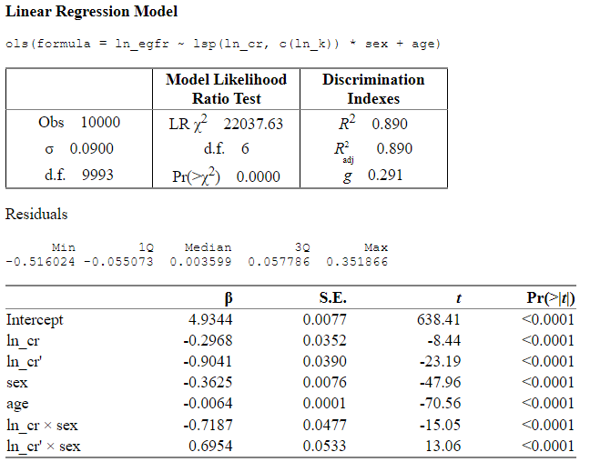
And this is how I would write down the full model in log or natural scale
# log scale
coef(fit)["Intercept"] +
  coef(fit)["ln_cr"]*log(cr) +
  coef(fit)["ln_cr'"] * pmax(log(cr/k), 0) +
  coef(fit)["sex"]*sex +
  coef(fit)["age"]*age +
  coef(fit)["ln_cr * sex"]*log(cr)*sex +
  coef(fit)["ln_cr' * sex"]* pmax(log(cr/k), 0)*sex

# natural scale
exp(coef(fit)["Intercept"]) *
  cr^coef(fit)["ln_cr"] *
  pmax(cr/k, 1)^coef(fit)["ln_cr'"]*
  exp(coef(fit)["age"])^age*
  exp(coef(fit)["sex"])^sex*
  (cr^coef(fit)["ln_cr * sex"])^sex *
  (pmax(cr/k, 1)^coef(fit)["ln_cr' * sex"])^sex
My main questions are
-
How did the authors end up with knot located at two different points using the same dataset (0.7 and 0.9 for female and male, respectively)?
Does this imply that they fitted the model separately for the two subgroups? -
In their equation, min(Scr/k,1)^α * max(Scr/k,1)^-1.209 is the term used to express the effect of creatinine. The left part is 1 when cr is above the knot and the right part is 1 when cr is below the knot. But if my understanding of linear spline is right, this is not how they are supposed to work (the first term should not be “null” when the variable is above the knot and viceversa).
Thank you very much.
There are many spline bases there are OK to use. The main question is does the model fit the data. I hope the original paper will explain the different knots.
A key question is why log? Why not a different transformation? What works best?
I’d also like to see residual diagnostic plots.
Note: to get math form of fitted model use latex(fit).
@f2harrell Thanks for your reply.
I know that by using latex(model) we can get the math of the model and I currently use it in quarto document. But this time I’ve written the model manually just to practise and be sure that I’m actually getting what I’m doing (my model development with the simulated dataset was just for practise as well).
What I find puzzling is how is possible to model log creatinine using a linear spline with one knot, while locating the knot at different point according to sex (0.7 for female and 0.9 for male). Dose this mean that they fitted the model separately for male and female?
I understand there many questions left behind about how they selected the functional form, evaluated the model fit and so on.
But now I’m just trying to understand what they actually did in the manuscript.
Thanks again for your reply and all the amazing teaching material shared on your website.
dear @f2harrell, I’ve just realised that my second question has no point and
min(Scr/k,1)^α * max(Scr/k,1)^-1.209 is a right way to explicitly report the linear spline.
Yet, I definitely can’t understand how they derived the spline locating the knot at two different place (0.7 for female, and 0.9 for male). Even if we introduce an interaction term between Cr and Sex we should derive a sex specific slope but the turning point (knot) should be the same.
Is my understanding wrong?
Thanks for your help, very much appreciated
1 Like
I think you’re right. A bigger question is does the linear spline actually fit? Why not use an equation that is smoother?
Thanks for your reply and your time. So, you agree that they must have fitted the model separately in male and female? Is this approach reasonable? I presume that keeping all data and modelling sex should be a much better approach.
As for the linear spline, they had a huge dataset so they could have used a smoother approach such as rcs.
The knot for the linear spline was picked up looking at the results of a non-parametric regression, isn’t this an example of double dipping?
I’d say that’s mild double dipping, which is less of a problem as N gets large. Fitting males and females together would have been a little better. There is another lack of fit test that should have been applied: make sure that SCr does not add to the prediction aside from how SCr is already included in the model.
1 Like
Thanks for your suggestion.
Unfortunately, I’m just revising the literature about GFR estimation and I don’t have raw data to check if Scr could have been modelled better.
Do you mean creating a new model with an additional SCr parameter and estimating the added information gained using various metrics as a method to check whether SCr was appropriately included in the original model? Very interesting. How is this not double dipping or a garden of forking paths problem with regard to choosing the modelling strategy of SCr?
Yes; perhaps not. It’s a goodness of fit test that involves the comparison of only two models so there’s not much model uncertainty. Example: if the main variables were just age and SCr you could add a tensor spline in (age, SCr) to their model and see if AIC improves. That’s a general goodness of fit assessment. I am a bit unconvinced that things are as linear as the accepted model would have you believe.
Dear Professor.
I’d like to inquire about methods for transforming the smoking variable into a continuous variable.
Participants are asked whether they are non-smokers, past smokers, or current smokers. Past smokers are further asked about the number of packs in the past, the duration of smoking, and the number of years since quitting. Current smokers are asked about the current number of packs and the duration.
My objective is to transform smoking into a continuous variable, rather than grouping participants into three categories (non-smokers, past smokers, current smokers), as you advised against the subgroup analysis. ![]() If this is a bad idea, please let me know.
If this is a bad idea, please let me know.
Non-smokers can be coded as 0, and current smokers can be coded as pack-years of smoking. However, coding for past smokers is challenging due to the involvement of past smoking quantity and years since quitting.
May I ask if you have any good methods?
Thank you.
(I’m not sure if this question is appropriate for this topic. If I’m wrong, please let me know where it should be)
I’ve been hoping that someone would publish a standard scoring rule that took all that into account. Perhaps you can find one. If it doesn’t exist and you have enough data you can build your own cigarette score, main effect for pack years and current status and an interaction between pack years and years since quit to allow for a decay function.
1 Like
Dear professor,
I am wondering if there is a suitable method to use whether implementing checks as an exposure factor.
I have observational data on a prospective cohort, including baseline measurements such as blood pressure and glucose, as well as data on cardiovascular disease incidence with 10-year follow-up. I’m considering whether to conduct fundus screenings for everyone or only for high-risk individuals (i.e., those with high blood pressure or high glucose). Screening everyone poses cost issues, so I want to demonstrate that screening only high-risk individuals can effectively predict future cardiovascular risk.
For instance, can interactive modeling like surv(py, cvd) ~ age + sex + fundus + highrisk + fundus:highrisk + (other_confunders) be effective? Here, ‘highrisk’ is a binary variable (0 or 1), with 1 indicating the need for fundus examination as determined by medical professionals due to high blood pressure or high glucose or other reasons. 0 means no fundus examination will be conducted (i.e., this group of individuals will not be examined in reality). Fundus is the results of fundus examination.
And, when I include a binary variable (highrisk) based on high blood pressure and high glucose in the model, can I also include the continuous values of blood pressure and glucose as part of the modeling? For example, surv(py, cvd) ~ age + sex + fundus + highrisk + fundus:highrisk + SBP + glucose. Would this lead to negative impacts on the model due to the relation between the binary variable (highrisk) and blood pressure and glucose?
First I would use binary logistic regression to model the relationship between the continuous variable that are supposed to be taken into account with ‘high risk’ and the actual high risk designation. See how redundant the high risk designation is, e.g., its the relationship between predicted high risk and designated high risk flat on one side. Then decide what to do.
1 Like
Dear Professor,
I have a question about predictions.
Below is a simple Cox model. I have plotted the predicted hazard ratios for age in males and females respectively.
The model does not include an interaction between age and sex, so I thought the predicted curves in males and females should be the same. However, the predicted curves in males and females are different.
I may mistakenly understand that the output of predict was calculated by the beta of age only. Is the output of predict the prediction of the entire model, that is, is the predict calculated by the beta of age and the beta of sex together?
Thank you very much.
require(survival)
require(ggplot2)
require(rms)
n <- 1000
set.seed(123)
age <- 50 + 12*rnorm(n)
sex <- factor(sample(c('Male','Female'), n,
                     rep=TRUE, prob=c(.6, .4)))
cens <- 15*runif(n)
h <- .02*exp(.04*(age-50)+.8*(sex=='Female'))
dt <- -log(runif(n))/h
e <- ifelse(dt <= cens,1,0)
dt <- pmin(dt, cens)
dd <- datadist(age, sex, bp)

options(datadist='dd')
S <- Surv(dt,e)
f <- cph(S ~ age + sex + bp, x=TRUE, y=TRUE)
f <- update(f)

#  predicted hazard ratios for age in males and females
ggplot(Predict(f,
               age,
               sex ="Female",
               ref.zero = TRUE,
               fun = exp), aes(age, yhat)) +  geom_line()

ggplot(Predict(f,
               age,
               sex ="Male",
               ref.zero = TRUE,
               fun = exp), aes(age, yhat)) +  geom_line()
Predict uses the whole model. Interaction is assessed on an unrestricted scale like the linear predictor in the Cox model (log relative hazard scale). When you nonlinearly transform that scale you’ll see apparent interactions but don’t be misled by that.
1 Like
Thank you very much ![]()
Professor Harrell,
How do I interpret the results from the model when my outcome is a z transformed variable (weight in z scores) and exposure (VitaminD) is log2 transformed ?
The summary estimates from the model are as follows.
 term                      estimate           s.error
> VitaminD                 -0.0000178         0.00023
> age                       0.1867            0.043
> VitaminD*age              0.00028           0.017
I don’t recommend z scores because of interpretation difficulties.
1 Like