The goal is to evaluate the impact of an intervention on children’s BMI before and after the intervention. Ideally, evaluations should occur at three distinct time points (t1, t2, t3). However, the available data exhibit unbalanced repeated measure design, some children evaluated only once during t1, t2, or t3, others assessed twice during t1/t2, t2/t3, t1/t1, t2/t2, and some evaluated at all three time intervals.
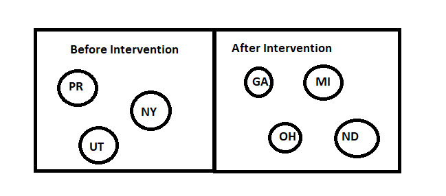
Additionally, this is a multi-center study. Not all centers provide both before and after intervention data. For before intervention, I have 100 observations from children in NY, 200 observations from children in Puerto Rico, 150 observations from children in Utah. For after-intervention period, I have data from children in Michigan, Georgia, and Ohio.
Given the clustered nature of the data and the mismatch between before and after intervention data across different centers, I am uncertain about the most appropriate model to fit. Would an autocorrelated time series model or a mixed-effects model be more suitable for this unbalanced repeated measure, multi-center intervention study?
Though it won’t solve all the problems with this study, a continuous time correlation structure (e.g. AR1) and a continuous time mean function (e.g., a spline in time) will help.
1 Like
Frank, In regression model when including baseline measurement as a predictor how do we handle scenarios where few subjects are measured only once and no followup measurement whereas several other subjects were evaluated twice once at baseline and second measurement sometime in the future.
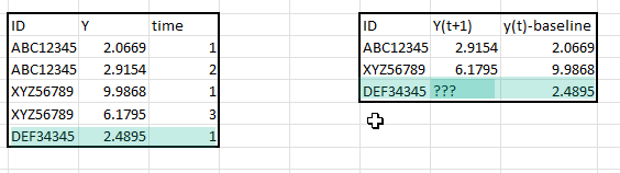
How should we handle this situation ?, Is it okay to do a LOCF (Last Obsv Carry Forward) for such cases where there are only baseline measurements and no followup ? Thanks in advance.
LOCF is almost never a good idea, and can’t be used unless you have at least 2 non-missing follow-up values. The observations without any follow-up data are only useful for unsupervised learning (data reduction) steps to help with high-dimensional predictors. They contribute almost no information. Multiple imputation will gain a slight benefit of having non-missing predictors but hardly worth the effort.
It is important to note that if you are trying to draw any conclusions from changes from pre to post, a pre-post design cannot withstand losing even a single observation because of missing follow-up. Pre-post designs are extremely brittle and non-response bias will ruin the analysis.
1 Like
Thank you Frank. I will plan accordingly. Probably start with only those with alteast two measurements.
That is likely to create a serious bias. Start with fitting a logistic model to predict the number of follow-up measurements based on all non-missing baseline data. And talk to the experts to see what features they think dictate a patient being followed.
1 Like
Great idea, did not think about model to predict the number of follow-up measurements, will do. Thanks as always.
Hi Prof Harrell,
I would like to ask regarding chapter 7.8.4 Bayesian Markov Semiparametric Model of the rms book.
(1)
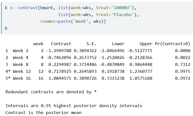
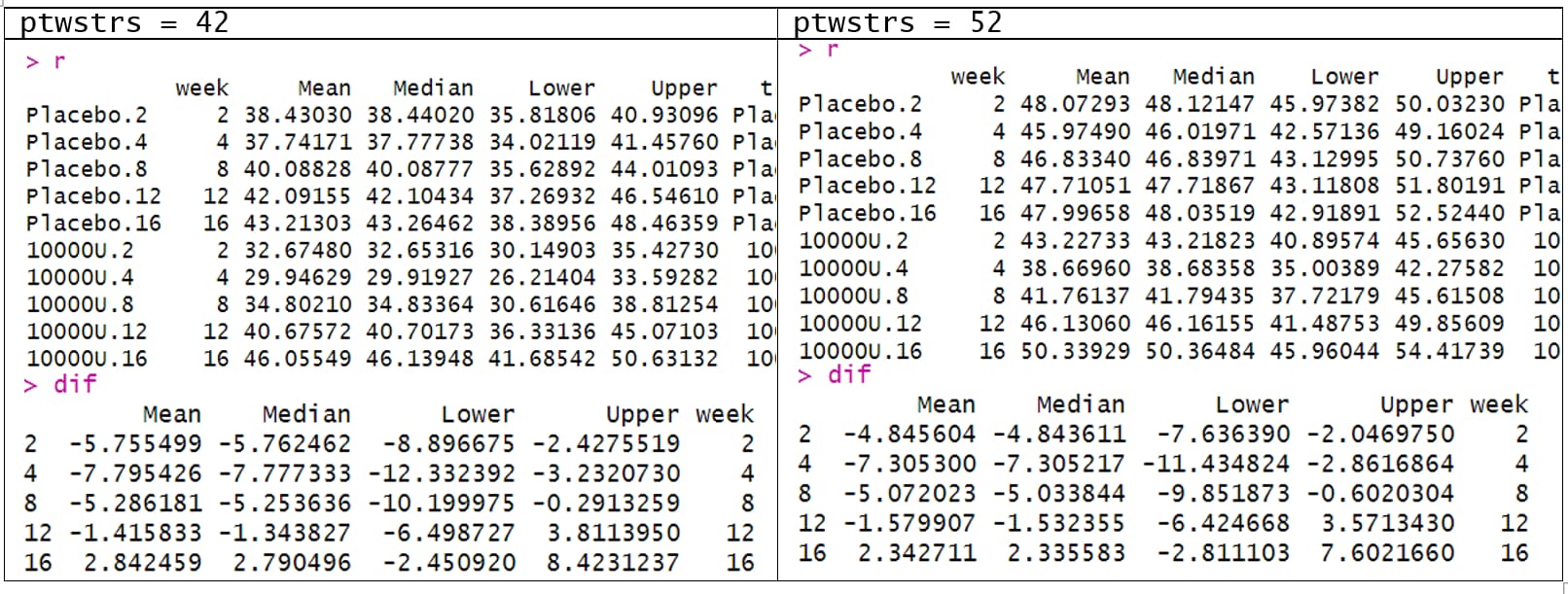
I have difficulty understanding what contrast.rms does to a blrm object. I have understood it to be the estimated difference in means between two groups, here, 10000U-Placebo, similar to the emmeans::emmeans and modelbased::estimate_contrasts functions.
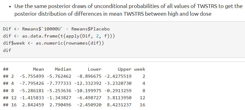
However, when I refer to the latter section, where the differences in mean is obtained from the unconditional probabilities, the values appear different.
How do I understand the difference in these two results?
(2)
Additionally, the contrasts are only for between-group differences at each timepoint. Would it be logical or meaningful to look at within-group differences, example, Week 4-Week 2, Week 8-Week 2 etc for 10000U and Placebo groups separately? Or would it be better to use conditional mean?
(3)
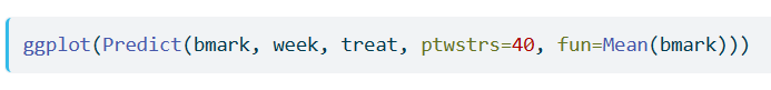
If we use conditional mean, the previous value, ptwstrs=40 needs to be specified. Is this value arbitrary?
Thank you for taking the time to read my questions!
The results have entirely different estimands. One relates to differences in log odds of transition probabilities and the other to differences in means (on the original scale) between two of the treatments at separate follow-up times.
It is possible to do that but it is not conventional when there are more than one follow-up times. We tend to look at between-group differences, slopes, curvature, etc.
Whenever estimating an absolute (not a transition odds, for example) you’ll need to define an initial state. It would be better to do this for 10 different initial values.
Thank you for clarifying!
If I understand this correctly, this is the same as log of transition odds ratio. Is there a way to code it directly in contrast so that I can get the transition odds ratio? I tried including the argument fun = exp like in logistic model, but it didn’t work.
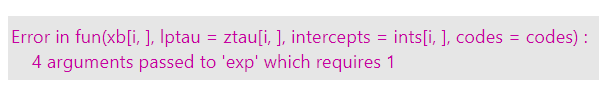
Set funint=FALSE in contrast().
Hi all,
I would like to ask further questions from 7.8.4 Bayesian Markov Semiparametric Model 1 of the rms book. Appreciate any help and guidance.
-
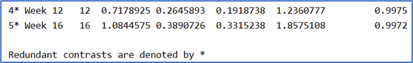
What does redundant contrast mean and how are they determined in the context of Markov models? Specifically, in the example, weeks 12 and 16 have contrasts of > 0 and corresponding higher posterior probabilities, but they are considered redundant?
-
There’s a section where subject-level random effects, cluster(uid) is introduced into the model. The random effects SD is small at 0.11, hence, we can simplify the model by omitting random effects. In my study, I ran the model 6 times for 6 different outcomes; one continuous and the others, ordinal with 3 levels. The random effects SD is small for the continuous variable i.e. 0.3, but the rest have bigger SDs between 1.7 and 2.7. Is it then necessary to run these 5 as random effects Markov model?
-
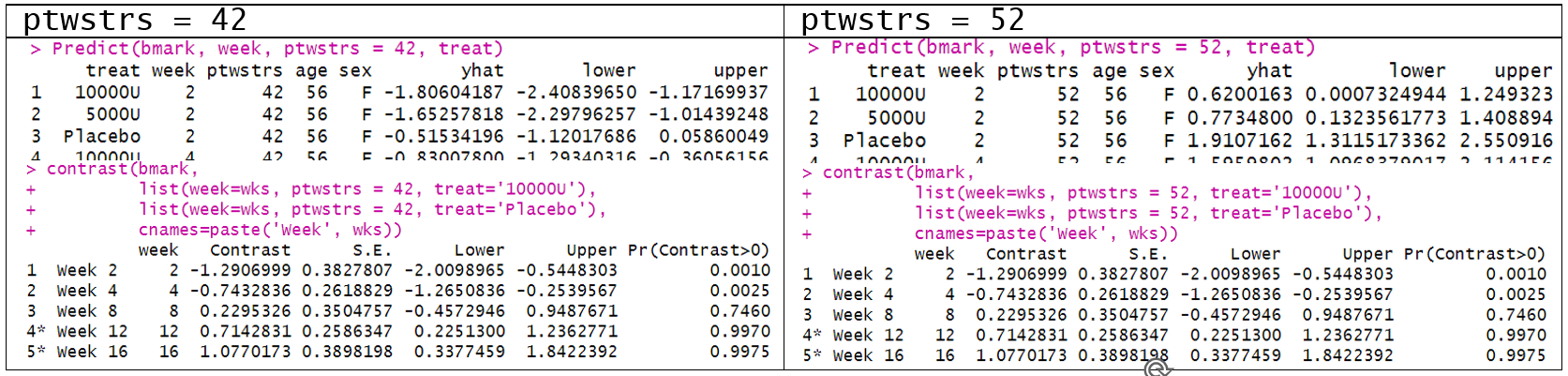
When we obtain the contrasts (as difference in log odds), the predictor settings do not matter. i.e. contrasts for when ptwstrs=42 is the same as ptwstrs=52.
But why do we need to set the predictor combinations for unconditional means? Also, are there posterior probabilities associated with the difference in the unconditional means?
Thank you!
Dear Professor @f2harrell,
In the rms pakage there is the function Gls() as the equivalent to gls() from the nlme package.
By using rms::Gls(), it is possible to use the many after-fit functions from rms, such as anova(), summary(), ggplot(Predict()), and contrast(), as shown in the case study from Section 7.8.
Is it possible to do the same with the nlme::lme() function?
Thank you.
No those methods have not been implemented for random effects models in rms. Look at the effects package for some possible solutions, and John Fox and Sandy Weisberg have an online appendix to their regression model that has some very general methods for plotting partial effects etc.
2 Likes
Ok, many thanks for the suggestions!
Does anyone know this paper by Jos Twisk?
Different ways to estimate treatment effects in randomised controlled trials (sciencedirectassets.com)
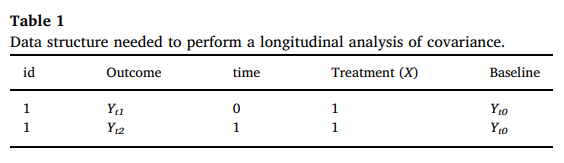
For a 2 parallel arms RCT with 3 assessment times (T_0, T_1, T_2) where the outcome variable is systolic blood pressure, the authors propose the following analysis approach:
The models are mixed effects models with a random intercept.
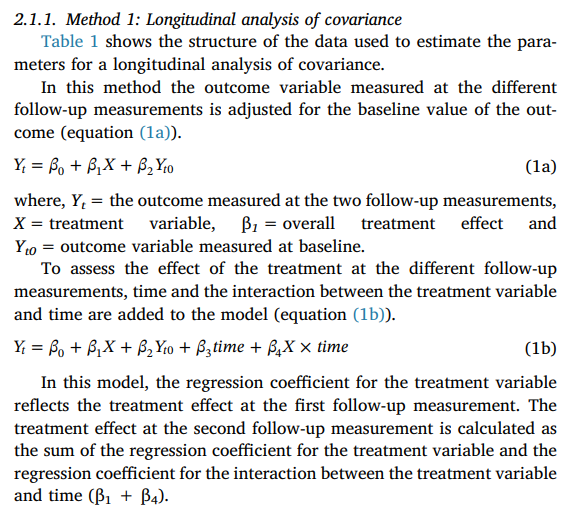
As the image above shows,
For model 1a,
\beta_1 is the overall treatment effect,
While for model 1b,
\beta_1 is the treatment effect at T_1 (first follow-up) and
\beta_1 + \beta_4 is the treatment effect at T_2 (second follow-up).
I’ve never seen this before.
Professor @f2harrell, what’s your take on this?
That is covered in detail in Regression Modeling Strategies - 7 Modeling Longitudinal Responses using Generalized Least Squares . It is not a good idea, the simplest reason being that depending on inclusion criteria the baseline measurement may have a truncated distribution thus requiring a multivariate model that has different distribution shapes for different times.
Thank you Professor.
With regards to Gls, does it make sense to use it when I have only 3 assessment times (baseline + 2 follow-ups)? In this case, should time be modeled as a continuous variable?
I’ve tried some simulations and when I compare different correlation structures (as in section 7.8.2 of the RMS course notes), the models yield all the same AIC.
With only 2 follow-up times and if all subjects are followed at exact the same 2 times the correlation structure doesn’t matter. If times are not all the same it’s best to model time and correlation continuously, then the different structures will give slightly different answers.