RMS Modeling Longitudinal Responses

Regression Modeling Strategies: Modeling Longitudinal Responses

This is the seventh of several several connected topics organized around chapters in Regression Modeling Strategies. The purposes of these topics are to introduce key concepts in the chapter and to provide a place for questions, answers, and discussion around the chapter’s topics.

Overview | Course Notes

Additional links

RMS7

1 Like

Q&A From May 2021 Course

  • What do you suggest for panel data? (longitudinal data with time discrete, as often occurs in patients’ registry). No difference. Can use continuous time methods for discrete time, perhaps only changing to an unstructured covariance matrix if there are 2 or 3 distinct times.
  • Longitudinal data includes 2 time points? 2 or more
  • What if patients were seen at different time-points (clinical routine)?How does it impact time-effect? Continuous-time models such as AR1 handle this nicely.
  • How do you decide whether a generalized least square or a mixed effect model fits better your data? Start with the variogram. For a standard mixed-effects models the assumed variogram is flat.
  • What is your preferred way to calculate R^2 and/or assess explained variance between fixed and random effects for mixed effect models? Haven’t studied that

Is there a way to run bootstrap validation and calibrate a gls model (fit using gls in the rms package)?

Sorry that’s not implemented.

1 Like

Dear Prof @f2harrell,

I’m trying to simulate some serial data to show the increased Type 1 error rate of analyzing it as if it were independent data.

For instance, I’m comparing the frequency of p<0.05 using OLS vs GLS when there’s no real association between X and Y. The relevant code is as follows:

x <- genCorData(n, mu = c(80, 80, 80),
sigma = 40,
rho = 0.7,
corstr = 'cs',
cnames = c('x1', 'x2', 'x3'))

y <- genCorData(n, mu = c(100, 100, 100),
sigma = 50,
rho = 0.7,
corstr = 'cs',
cnames = c('y1', 'y2', 'y3'))

Gls(y ~ x, data = data, correlation = corCompSymm(form = ~ measure|id)))

Note:

  • “cs” above stands for compound symmetry.
  • I’m running 1000 simulations of 10 subjects with 3 (x,y) measurements each.

The frequency of p<0.05 is ~ 8% for GLS and ~ 20% for OLS.

Isn’t the first one too high?

I’ll bet that the normal approximation for \hat{\beta} is not great for N=10. The p-value would probably be good were a t-distribution to be used instead of Gaussian.

Thanks.
Do you mean that the fit of the GLS model is suboptimal in terms of achieving normally distributed residuals? Or, alternatively, that the data generating mechanism should be based on sampling X and Y from a t rather than a Gaussian distribution?
Apologies if I’m not following…

Neither. Take the special case of GLS with one time point. Then GLS=OLS and we use the slightly wide t-distribution for getting p-values instead of the normal distribution.

Is there a way to do that using the rms package?

I’ve come across the parameters package:

We can select a t-distribution approximation for computing p-values and confidence limits of regression coefficients:

parameters(f, ci = 0.95, method = 'residual')
Parameters

Is that what you mean?
Unfortunately it does not seem to work for Gls models.

To solve my problem from the message above, I simply increased the sample size from 10 to 30 and now the frequency of p<0.05 is 5.5% with Gls, which seems correct.

The parameters idea is restrictive. A lot of hypotheses are on linear combinations of parameters and involve > 1 degree of freedom. Hence the contrast function in rms. It does’t provide t-based p-values for gls though.

1 Like

Hi!

I have longitudinal data of abdominal surgery patients at 4 timepoints (baseline, 1-month, 3-month, 6-month). The response is the EQ visual analogue scale (EQ VAS), which ranges from 0 to 100. The 3 groups for comparison are mild-to-moderate anemia, mild anemia and non-anemia. I have used the generalized least squares and followed the guide from the rms book/short course.
Here is the code that I have used.

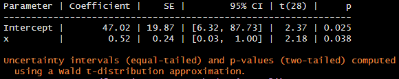
a <- Gls(vas ~ anemia * month +
           vas0 + rcs(age, 4) + sex + type + lap_open, data=df, 
                correlation=corCAR1(form = ~month | ic))

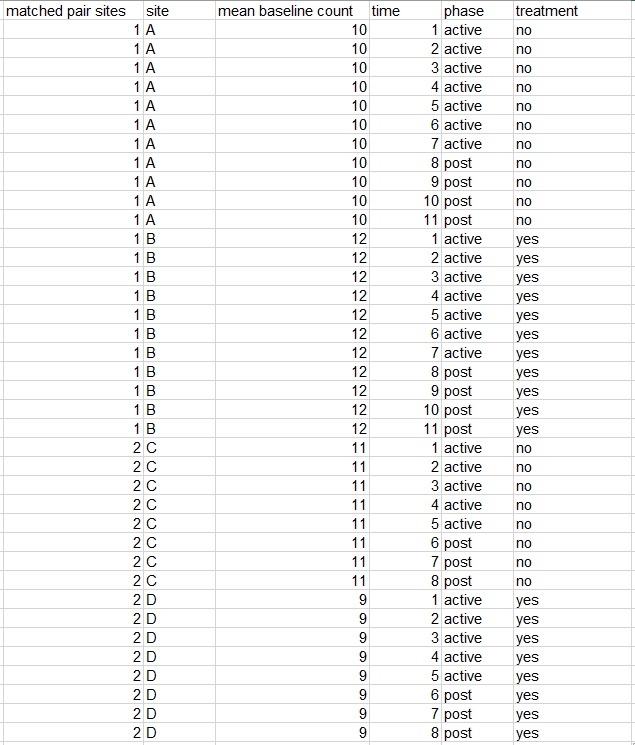
where, vas is the vas score at follow-up (i.e. 1-month, 3-month and 6-month), anemia is the 3-level severity of anemia (i.e. mild-to-moderate anemia, mild anemia and non-anemia), month is integer value (i.e. 1, 3, 6) vas0 is the baseline vas score, age is age of patient at baseline, sex (female, male), type is either gastro, hepa or uro/gynae, lap_open (i.e. either surgery is laparoscopic or open) and ic is the unique patient identifiers. I assume linearity for month. In the book, it stated “Time is modeled as a restricted cubic spline with 3 knots, because there are only 3 unique interior values of week.” Here, what does it mean by interior values?

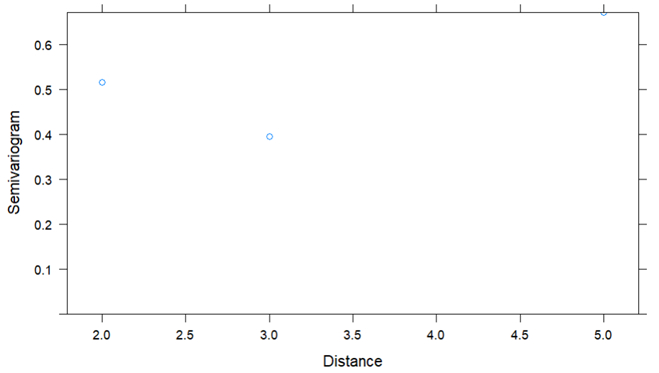
When I plot the variogram, it gives me only 2 points. How do I assess this?

image

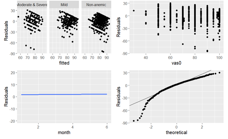
When I plot the variance and normality assumptions, the residuals do not look random and the qqplot does not seem to follow the theoretical normal distribution. Does this suggest that I abandon the GLS? What statistical method should I use here?

Besides EQ VAS, I would also like to look at the individual domains of the EQ-5D-3L (ordinal variable with 3 levels) and utility score (range from 0.854 for state 11121 to -0.769 for state 33333). Would it be useful to look at Semiparametric Ordinal Longitudinal Models?

Thank you!

2 Likes

Nice work. For the types of outcome variables you have, it is common to see floor and/or ceiling effects as you see in your residual plots. Ordinal models typically work much better. This is a case study that should help, as your situation seems to go along with a Markov process.

I am finding that the baseline needs to be nonlinearly modeled (using e.g. a restricted cubic spline) for these types of outcomes because some patients can start off at extremely bad levels and get major benefits from treatments.

The variogram has only two points because the x-axis relates to time gaps and there are only 2 distinct time gaps in your data.

A major problem: Anemia doesn’t exist in 3 distinct states. It is a continuum. The underlying hemoglobin or hematocrit should be used, continuously.

3 Likes

Does anyone know how to perform a sample size calculation for a 2 arms RCT with 3 assessment times (baseline, end of treatment, and follow-up) analyzed with Generalized Least Squares (rms::Gls)?

Any specific packages? Thank you.

Try Selecting a sample size for studies with repeated measures | BMC Medical Research Methodology | Full Text and especially http://dx.doi.org/10.1198/tast.2009.08196 - compute the effective sample size per subject and use traditional methods to estimate number of subjects, then divide by effective sample size per subject.

Hi!
I’m new here so forgive me if I’m posting in the wrong section of the forum.
We have monthly longitudinal count data (uptake of a clinical intervention) for baseline, active intervention phase and post intervention phase for 12 sites. 6 of these sites are controls which do not receive the intervention, each of which is matched to a treatment site. The number of months worth of data differs between sites - for example one site might have 3 months of baseline, 10 months active intervention and 4 months post intervention, whilst another site might have 2 months of baseline, 12 months active intervention and 6 months post intervention. However, the matched pairs of sites have the same longitudinal structure.
It appears like the generally preferred approach is ANCOVA type, where baseline Y is included as a covariate. However, I’m uncertain of the best modelling strategy to make use of all the data available.
My initial thought is something like:

Y(i,t) ~ intercept + baseline(i) + time * phase(i,t) * treatment(i) + covs(i,t) + (1|site)

where Y is the count at site i at followup time t, and baseline is the MEAN of several months of baseline Y. So for each site, Y at each followup month has the same baseline. time is followup time, beginning at start of intervention and phase is categorical (either active- or post- intervention). The control sites are specified as either in the “active” phase or “post” phase though of course they don’t really receive the intervention. treatment is binary indicating whether the site is a treatment- or a control- site. covs is other covariates of interest e.g. sex etc. site is a random effect term. I plan to model baseline and time as continuous variables using splines. Error distribution will be something like Poisson or negative binomial.
I would greatly appreciate some thoughts on this. Particularly, I was unsure about how best to incorporate several months of baseline data (above I used averaging), and also that for the phase variable, “post” always comes later in time - will this cause any problems? Im also pondering on whether there might be the need for several time scales - i.e. time since start active phase, time since start of post phase which might mean we no longer need the “phase” variable.

Here is how the data would be set up (only four sites shown hence 2 matched pairs)…

1 Like

Thank you professor, I will have a look at these references.

I found this code, from the longpower package (CRAN - Package longpower):

  • Description
    This function performs the sample size calculation for difference in slopes between two groups. See
    Diggle, et al (2002) and package vignette for more details.

  • Usage
    diggle.linear.power(
    n = NULL,
    delta = NULL,
    t = NULL,
    sigma2 = 1,
    R = NULL,
    sig.level = 0.05,
    power = NULL,
    alternative = c("two.sided", "one.sided"),
    tol = .Machine$double.eps^2
    )`

  • Arguments
    n = sample size per group
    delta = group difference in slopes
    t = the observation times
    sigma2 = the residual variance
    R = the working correlation matrix (or variance-covariance matrix if sigma2 is 1). If R is a scalar, an exchangeable working correlation matrix will be assumed.
    sig.level = Type I error
    power = power
    alternative = one- or two-sided test
    tol = numerical tolerance used in root finding

It seems straightforward. Any important considerations/caveats?

Thank you.

1 Like

You are thinking carefully about this and laying things out well. Without having a lot of “replicate” sites the design makes it hard to separate site effects from intervention effects so the inference will be very model-dependent I think. I hope others more experienced with this type of design will add more. Regarding baseline, it’s often best to adjust for multiple baseline variables, e.g., the last measurement, the average of all measurements, Gini’s mean difference of all baselines (if variability of baselines is interesting), slope of baselines over time. You might pick 2-3 of such summary measures.

Thank you Frank. Regarding your last suggestion of possibly including “slope of baselines over time”, did you mean an interaction term between time and one or more of the baseline variables?

Also, I wasnt sure if this is the best place on the forum as it seems to be a thread of replies, albeit concerned with longitudinal modelling. I can leave it here, but if you think the question might gain more attention somewhere else on the forum please let me know. Thanks!

It’s not a bad place for it but at some point we need a new topic on handling multiple baselines whether Y is multivariate or univariate. By slopes I was not referring to what you wrote but by fitting a line to each subject’s baseline measurements and using the estimated slope as a new covariate. Sometimes we summarize multiple baseline with multiple quantiles, sample entropy, or mean absolute consecutive differences to quantify general volatility.

Thank you Frank, I understand what you meant now.
Ive been thinking more, and believe that I might need to add another “time” predictor. So the model would have the currently used time variable (from start of active intervention) and there will be another time variable begining at start of post intervention. This column in the data will be a sequence of 0’s up until start of post phase upon which the clock begins. That way we can get conditional estimates for specific times since start active / post phase e.g. mean count 3 months after end of active phase. Do you think this is reasonable?