It’s not working. Not sure I can do it, as I’m not acquainted with R. Only started using it 2 weeks ago. I’m not an analyst/biostatistician. Therefore, overall, I’m pretty happy to have got this far (performing ols reg with rcs in R!). Thanks to you and your book, largely.
Anyway, I have another quick question:
I’ve built 2 Models, both with the same predictors (3 continuous and 3 categorical). Used 3 knots in one Model and 4 knots in the other. Which Model should I choose? RMS says something about maximizing the value of the “LR test - 2k”. Does that mean I should simply calculate “LR test - 2k” for each Model and then choose the Model yielding the highest result?
I suggest being patient and taking more time to read the RMS book or course notes. You’re learning R well. Biostatistics is not a topic that can be covered in a crash course.
Regarding the number of knots, RMS gives you some guidance. This should be pre-specified based on subject matter knowledge of effect shapes and based on the sample size. More sample size allows more complexity. Don’t base number of knots on a comparison like the one you outlined. That applies only to the whole model where lots of variables are splined and you feel they should all have the same number of knots (for some strange reason).
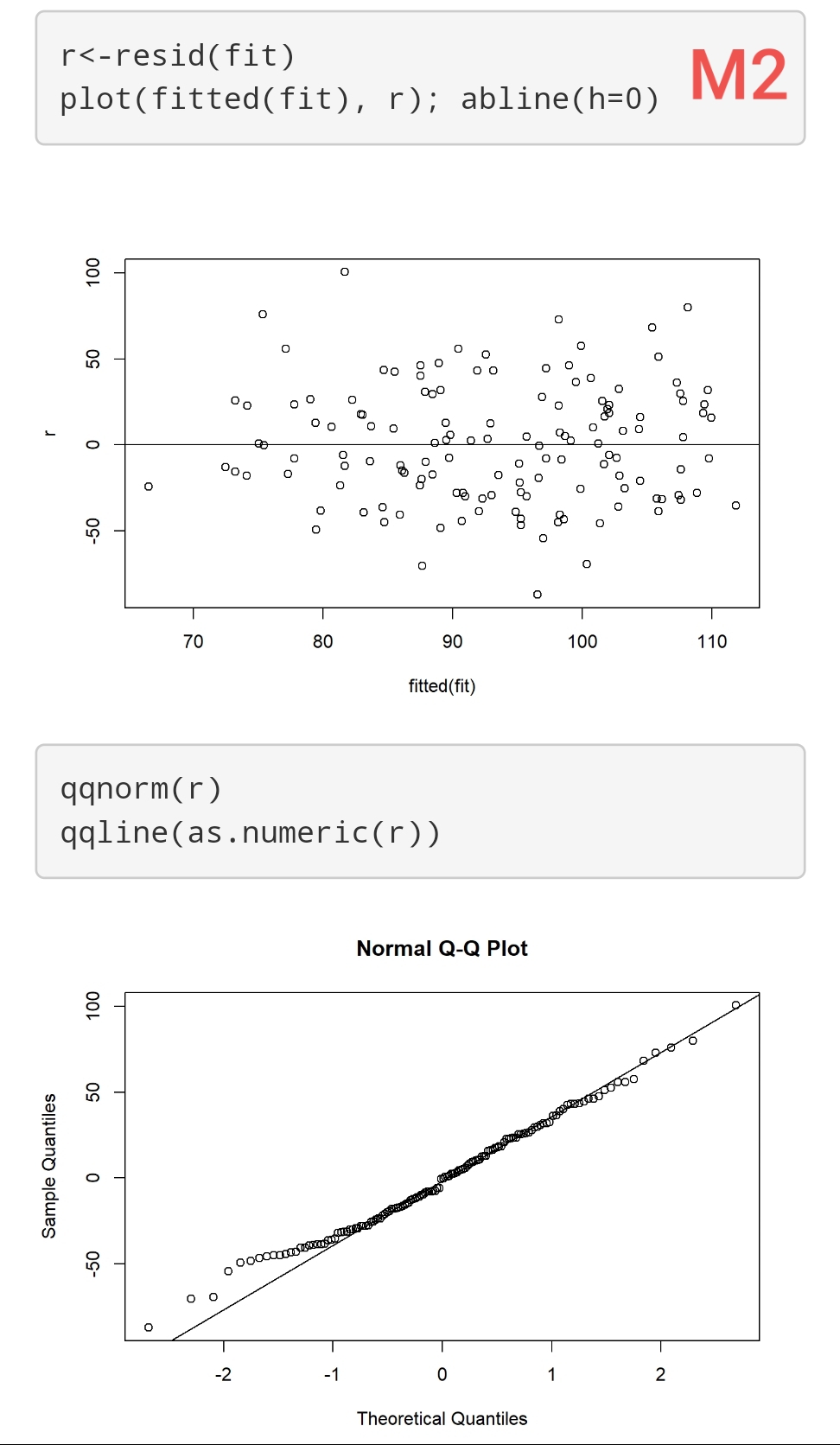
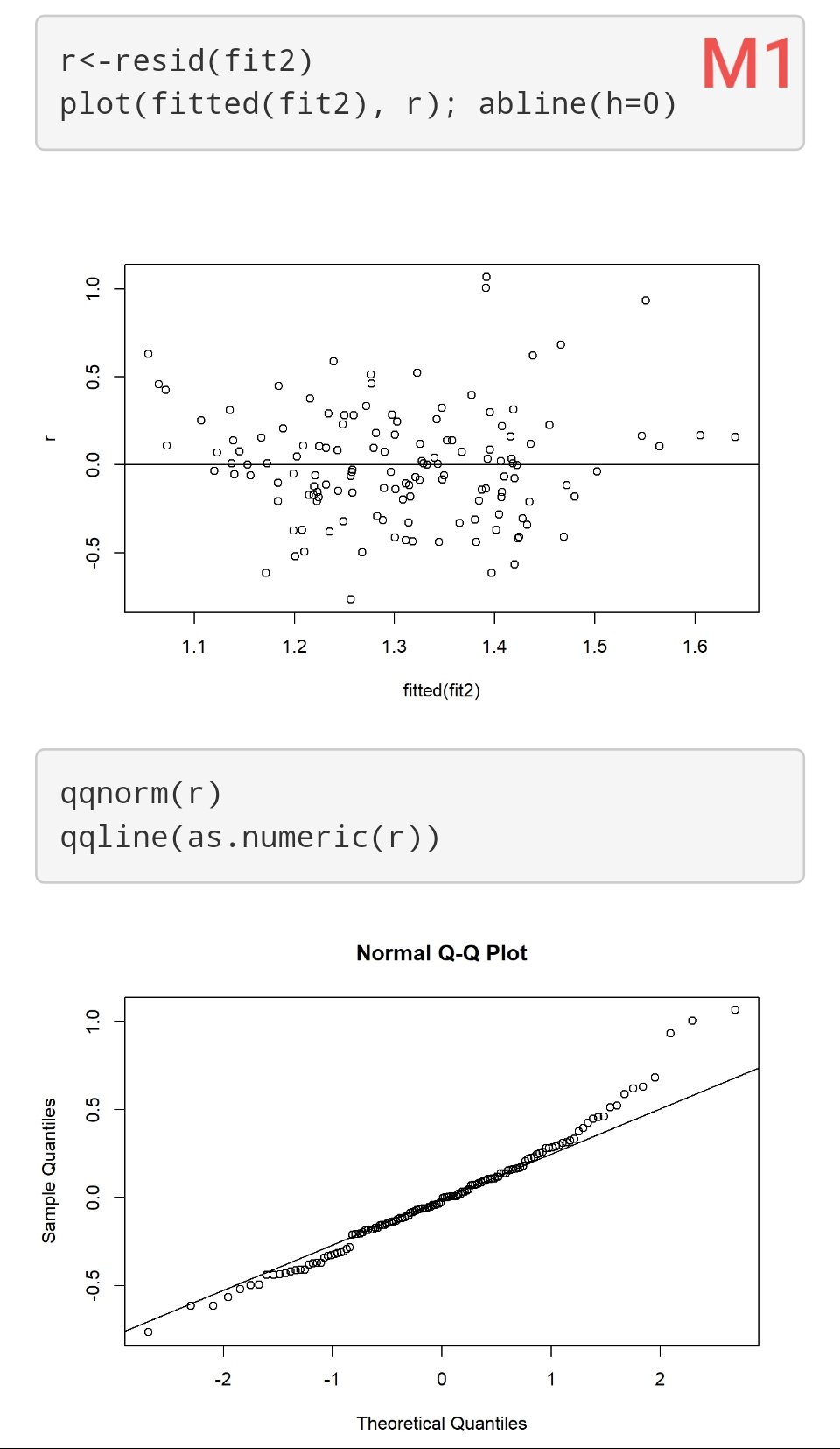
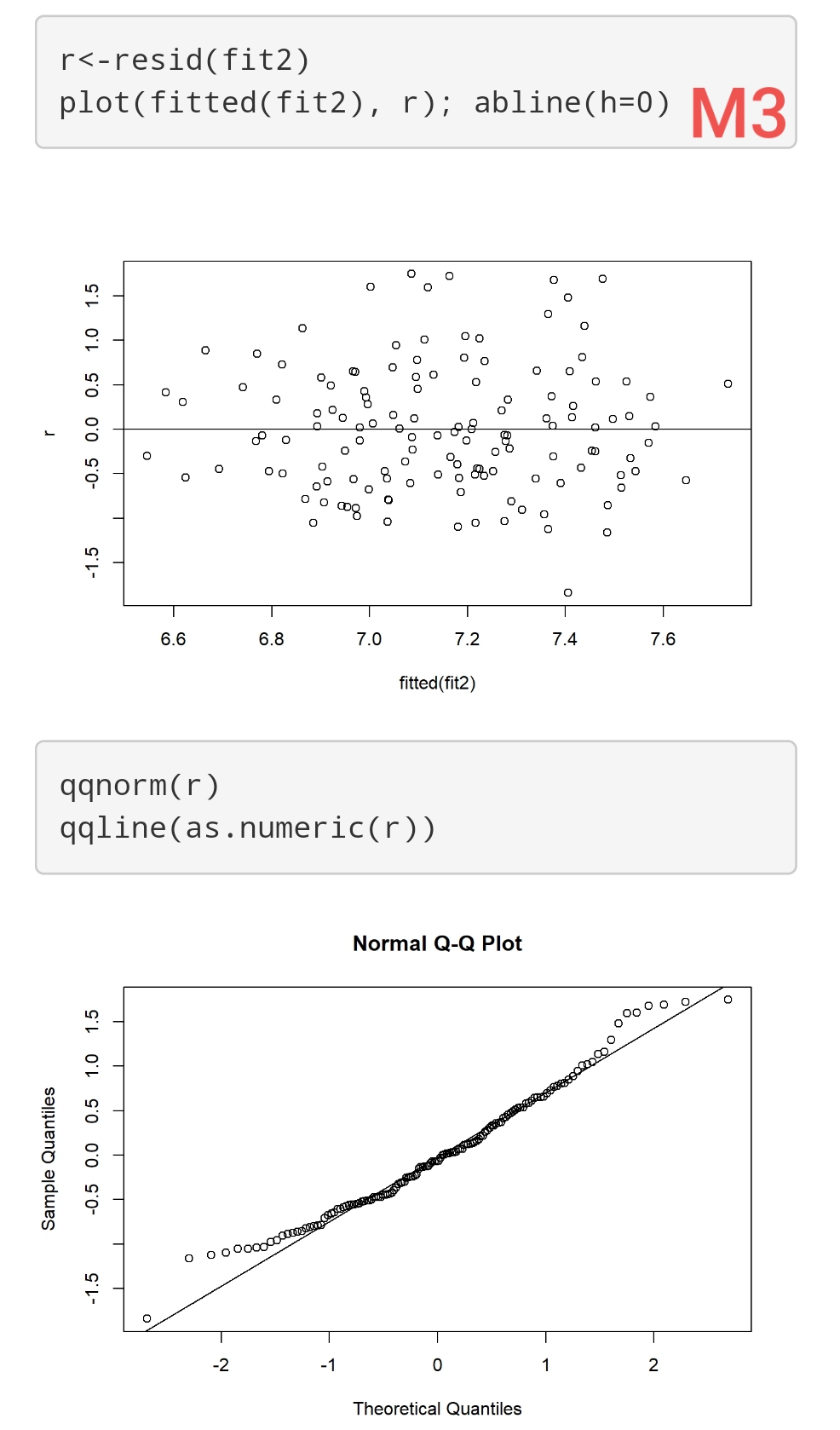
I have 3 Models (using ols reg with rcs). Their respective residuals are attached (M1, M2, and M3). Sample size is 140.
How “bad” are these residuals? It seems that homogeneity of variance is ok, but maybe there are problems with normality? However, they don’t seem to indicate major violations of this assumption (imo!). How would this affect the inferences from these models? E.g., results from “anova(f)” and “summary(f)”?
A question on variable clustering for feature selection:
I have a metabolomics dataset in which many of the variables are highly correlated. This is expected because the same metabolite can be detected at slightly different mass-to-charge (m/z) ratios and can occur in both the positive and negative mode.
My ultimate goal is to regress a biological outcome with a set of reduced features so that this reduced feature set can represent a set of biomarkers.
Thus, it is desirable to reduce the dataset so that highly correlated variables are represented by one single variable. I thought about using variable clustering for this purpose but I am unsure how to implement what I’d like to do.
I’d like to create synthetic variables (i.e., a cluster) where the members that compose the synthetic cluster all have a correlation of a minimum specified value to the synthetic variable itself.
For example, in a dataset of 1000 variables, I create 40 clusters each with on average 10 variables, and the variables within each of these clusters all have a pearson correlation of > 0.9 to the synthetic variable (can also be another metric, this is just hypothetical).
I can then drop all members of all clusters from the original dataset, retaining only the synthetic variables. If the synthetic variables are selected during the feature selection process, I can use members of the cluster in a reduced feature set instead of the synthetic variable.
I have checked both varclus and ClustOfVar but can’t see in either of these the possibility to do what I’d like. Usually, the number of clusters is specified based on the elbow method or visual assessment of plotted trees, however in my case this is obviously not unsuitable.
Does anyone have any advice on how this can be implemented?
These are good questions. You may find some useful discussion in stats.stackexchange.com. I find the whole model checking topic to involve too much subjectivity and also feel that we should concentrate on the more difficult task of assessing the impact of model departures. For example you could simulate 1000 datasets like yours and look a confidence interval coverage (both tails) when residuals are a little non-normal. I find that we read into diagnostic plots what we want to see, and it depends on our energy level that day. A better approach overall is to use models that assume less. For example, semiparametric ordinal models will result in the same regression coefficients no matter how you transform Y, and are robust to outliers in Y.
Chapter 4 or RMS covers several techniques related to your question, and another chapter has a case study in the promising approach of sparse principal components. Beware that when the sample size is not huge, any decisions you make about simplifying the data or projecting multiple variables into fewer dimensions may be highly unstable and non-reproducible. Try bootstrapping the process you want to use to get a stability analysis. In terms of your seeking a more automated process I don’t know of one right off hand. But sometimes it’s better to use highly penalized regression on the whole set of predictors without trying to partition the predictors. Of course if you had subject matter knowledge for partitioning the variables without using the data at hand to do so, then you’re really getting somewhere.
Thanks a lot for the response Professor. I have read Chapter 4 carefully (it led me to using variable clustering) so thanks for that! sPLS is also often used in metabolomics literature and I’ve considered using it. I also used Lasso for a similar purpose. For stability, I repeated my procedures with multiple repeats of CV. It seems there isn’t an option to do what I want then. So far I just guessed a conservatively high number of clusters and that did something similar to what I want, but obviously there’s guess work involved here. Anyway, thanks a lot for taking the time.
Thank you very much for your reply.
Will have a look at these references!
While searching the literature for further study material, I came across this paper:
It seems a very simple intro and tutorial on splines, which might be good for someone who is new to the subject and has only basic statistical background, like myself for instance. The problem is that I have no subject matter knowledge to judge the quality of such material. Does it look like it has good quality or is trustuworthy?
In the ‘print()’ output of rms there’s the result of a LR Chi-square test. Is this a test of the overall significance of the model? I’m asking because some standard statistical software report the result of an F test instead.
Also, is it correct to say that the adjusted R2 is a measure of model fit?
Tests don’t test “significance” but rather null hypotheses. The LR \chi^2 tests the global null hypothesis that no predictors are associated with Y. F is used for ordinary linear models only, and I elected to use LR for OLS to help people compare with other models. There is a 1-1 transformation between F and LR for OLS.
R^2 is not a measure of model fit. It is a measure of explained variation in Y also called predictive discrimination.
I still have a few questions regarding the interpretation of ols models using rcs (from rms package). I would very much appreciate if you could help me with these questions:
I’m primarily interested in testing and describing (linear vs nonlinear) the adjusted association between a predictor variable X and a response variable Y. Therefore, when looking at the output from my model, I think I should focus on the results of the anova(). More specifically, on the multiple degree of freedom test of association. Because I’m using 3 knots for X, I have 2df. The anova shows that the 2df test is statistically significant, and also that the 1df test (nonlinear) is also statistically significant. Does that mean that the relationship between X and Y is completely nonlinear or it is linear and nonlinear for different values of X? The reason I’m asking is because the two betas of X (X and X’) are significantly different from 0, according to the output from print().
Following up on the above question, what does it mean when the betas of a given predictor, in this case with 4 knots (X, X’, X’'), are not significantly different from 0 (output from print()), but the anova shows an association between X and Y through the multiple degree of freedom tests? In this case, both the 3df and 2df (nonlinear) tests are statistically significant.
I’ve learned from you that we should interpret the plot of the adjusted relationship between X and Y (ggplot(Predict()) only if the multiple degree of freedom test of association from the anova() is significant. Is this the test with the highest df? For example, for a given X with 3 knots, the anova shows the results of a 2df test and a 1df (nonlinear) test. In this case, if both are statistically significant, then we turn to my question number 1 above. If the 2df test is significant, but the 1df (nonlinear) test is not, then the relationship is linear and this should be reflected on the plot, correct? If the 2df test is not significant, then there’s no assocation between X and Y and we should not try to interpret the plot, correct?
You can’t tell from the anova. This is not the best approach. Focus on the graph and its confidence bands. And there is little reason to test for linearity.
Don’t even look at that. It’s arbitrary to the choice of basis functions.
I don’t think I said that. The plot is meaningful in all cases. The multiple d.f. test just gives you more license to interpret the plot.
In my field of research, it is quite common to use linear models to regress an outcome on a exposure. Many papers contain something on the line of the following:
We fitted generalised additive models (GAMs) to assess departures from linearity in the relationship between exposures and each outcome. If the effective degrees of freedom were equal to 1, the relationship was closer to linear.
This is kind of a justification to use, e.g., lm or a semiparametric model. I came upon the comments of a reviewer of a paper using data-adaptive methods like random forests, saying that there is no reason to use more complex models if there is no evidence of non-linearity.
I guess there are two scenarios:
Single exposure models (plus confounders)
Multi-exposure models (plus confounders).
I have the feeling that in the first case maybe this sort of test is appropriate, but what if there are interactions that are not camptured?
With GAMs most users set the degrees of freedom, and d.f. is not something that is solved for by the GAM. So the linearity assessment is a self-fulfilling prophesy if using GAMs in the usual way.
“If there is no evidence of non-linearity” involves two problems: the absence of evidence is not evidence for absence error and distortion of statistical inference. If one even assesses linearity assumptions it implies that non-linearity is entertained. Entertaining non-linearity, i.e., given the model a chance to be nonlinear, needs to be accounted for in confidence intervals, p-values, and Bayesian posterior distributions.
If you don’t know beforehand that the model is simple, it’s best to allow the model to be flexible, have more parameters (possibly with penalization or Bayesian shrinkage priors), and stop there. That approach will give you the correct, wider, confidence intervals and posterior distributions.
I see the importance of accounting for entertaining non-linearity. The rationale for this presented in the Grambsh & OBrien reference in Regression Modeling Strategies discussed inflated type 1 error, which makes sense in a Frequentist framework. I’m a little confused on how it translates to a Bayesian framework though. I understand that accounting for uncertainty is still important, but in a Bayesian framework I thought peeking at data and type 1 error are less important. Can you elaborate on the rationale for not evaluating for linearity (e.x. scatterplots) before modeling in a Bayesian framework?
It’s surprisingly similar. Ignoring pre-looks at the data will result in posterior distributions that are too narrow, i.e., overconfident, when the final model has fewer parameters than the most complex entertained model. Like the frequentist approach if you ignore previous steps when computing uncertainty intervals the results are completely conditional on that model being right.