Regression Modeling Strategies:
This is the 12th of several connected topics organized around chapters in Regression Modeling Strategies. The purposes of these topics are to introduce key concepts in the chapter and to provide a place for questions, answers, and discussion around the chapter’s topics.
Elinder & Erixson (2012, PNAS) provide the data on 18 maritime disasters since 1855, including the Titanic. They provide the data, over 15,000 cases & 17 variables (free at PNAS: https://www.pnas.org/content/109/33/13220). The Titanic is one of two disasters (the HMS Birkenhead is the other) in which female survival is greater than males From the abstract: “Women have a distinct survival disadvantage compared with men. Captains and crew survive at a significantly higher rate than passengers….Taken together, our findings show that human behavior in life-and-death situations is best captured by the expression “every man for himself.””
Additional links
RMS12
Q&A From May 2021 Course
- Table 9.2 Lines: can you comment/explain how to properly interpret each line and what information these give to understand the model?
age x sibsp (Factor+Higher Order Factors) 10.99 4 0.0267

Nonlinear 1.81 3 0.6134

Nonlinear Interaction : f(A,B) vs. AB 1.81 3 0.6134
1.81 = 3 d.f. Chunk test for the nonlinear interaction effects; In this case this measures the departure of interactions from being a simple product. 10.99 is the chunk test with 4 d.f. For all interaction terms involving age and sibsp. There is an option for the anova print method to have it tell you exactly which parameters are being tested.
→ extra Q: What are the hypotheses here? For nonlinear and nonlinear interaction (and also for TOTAL NONLINEAR, TOTAL INTERACTION). How should we interpret the p-values here?
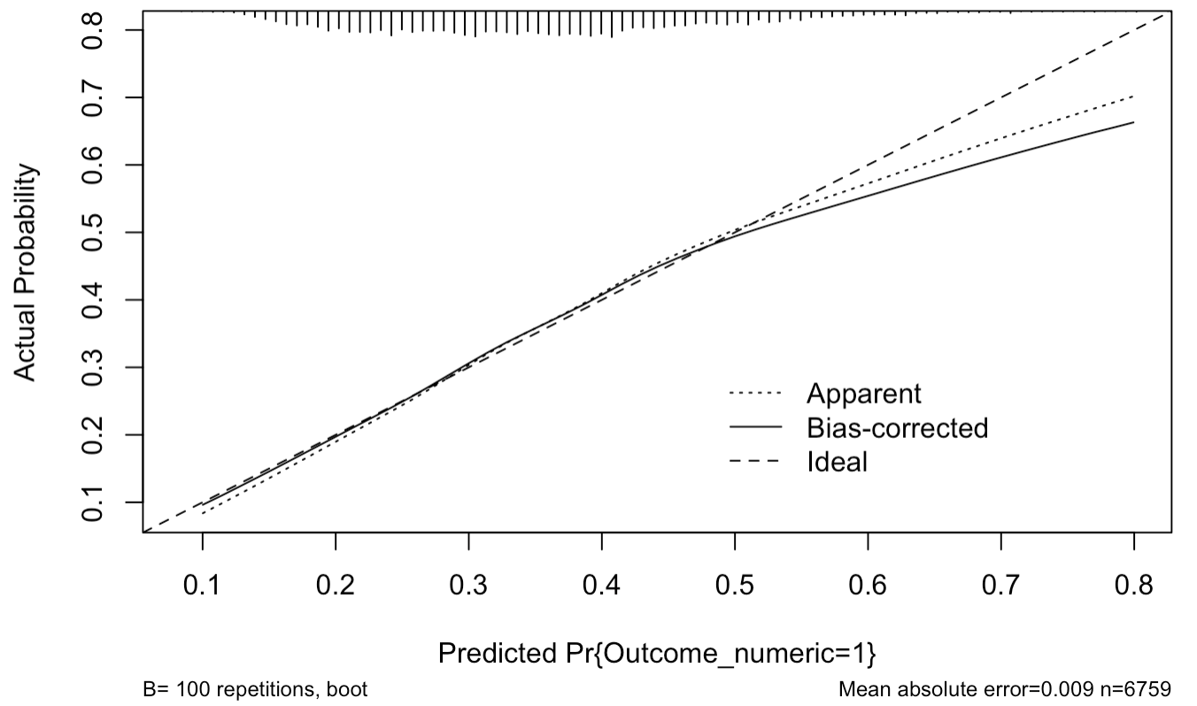
- Suppose I had a calibration plot looking like this:
Should I be concerned? Or is the lack of calibration at higher predicted probs OK as there are few data points there? Is there anything that can be done to improve the situation? Not too concerned. Mainly be concerned when prob = .55 .7 where you still have some data.
dear prof
I would like to know the option for that in anova print method.
thanks in advance
require(rms)
?print.anova.rms    # shows help file; see the argument called which
1 Like
Dear Professor Harrell,
I am trying to reproduce the code from cap 8 of your amazing book (case study on Titanic binary logistic regression).
Unfortunately, when I try to run this code chunk:
runmi ← function()
fit.mult.impute(survived ~ sex * pclass * rcs(age, 4) + rcs(age, 4) * (sibsp + parch),
lrm, mi, data=t3, pr=FALSE, lrt=TRUE)
seed ← 17
f.mi ← runifChanged(runmi, seed, mi, t3)
I get the following error:
Error in runifChanged(runmi, seed, mi, t3) :
attempt to run runifChanged without file= outside a knitr chunk.
could you help me? I am actually interest in fitting a cox regression model. In this latter case, would it work to change lrm with cph and swapping ‘survived’ with a Surv object?
Let me thank you for your help. I am apologize in advance in case the question is not posted correctly
Marco
This is one of those cases where my error message actually tells you what’s going on 
You are running the code interactively and not using knitr or quarto to run the whole document. For that cast you need to specify file= to runifChanged, e.g., file="my.rds".
The Titanic dataset does not have survival time; it only has survival as yes/no, so a survival model is not appropriate.
1 Like
Dear Professor,
Thank you very much, that worked perfectly for the titanic dataset!
Yes, my goal was indeed to translate the procedure applied in the titanic case study to a survival analysis. I would have used the case study on cox regression but in the latter only single imputation via transcan is used and in my dataset probably multiple imputation is advised.
That being said, I have tried to adjust the code for a survival analysis (like the prostate database) using cph instead of lrm.
To be more clear:
Model: 10 predictors (1 continuous and 9 factors) + time + binary outcome
S1 is the surv object from (time, outcome =1)
Example code:
set.seed(17) # so can reproduce random aspects
mi ← aregImpute(~ predictors + I(time) + outcome,
data=t3, n.impute=20, nk=3, pr=FALSE)
mi
runmi ← function(){
fit.mult.impute(S1 ~ predictors,
cph, mi, data=t3, fitargs = list(x=TRUE, y=TRUE), pr=FALSE)
}
seed ← 17
f.mi ← runifChanged(runmi, seed, mi, t3, file = “my.rds”)
could this be ok?, should i specify surv=true?
I can move this post to another tread if required
Thank you very much
Marco
That looks OK I think but my functions have only thought through the \beta part of the process, not the survival curve part. You may want to estimate the underlying survival curve by stacking all the imputed datasets. See this.
Thank you very much! Am I getting it right that I should use vClus to stack the imputed data sets and then draw the survival curve? Is this made within vClus or giving vClus output to survplot?
Thank you very much
Marco
You’ll probably have to look inside the functions I’m calling to see how it’s done.
I have a basic question regarding clustered data:
If we fit a blrm() model on clustered data using cluster(). (e.g., repeated measurements and we think they are exchangeable), and use the predict from from rms/rmsb, it sets the random intercept to 0.
Am I right that these are then predictions for a typical observation?
When the prediction model will be used for a new patient, I assume we should integrate out the random effect?
If we create calibration plots, should these then also use predictions where we integrated out the random effects?
Here the authors just set the random effects to 0 because they were tiny, but if they are not, what would the recommended approach? MC integration would obviously work, but that would takes a long time…
This has been address on the Stan discourse forum, I seem to remember, where an approximate technique was used for the marginalization over the random effects. I hope someone will respond who is more experienced about random effect Bayesian models. My sense is that for estimates on the link function scale (e.g., predicted log odds, odds ratios) setting random effects to their mean (zero) is OK, but for probability-scale estimates we need to marginalize. That would include calibration curves. I took the easy way out.
1 Like
Thanks. I found this thread which is helpful.
I quote Joshua Wiley.
Averaging over fitted values incorporating random effects does not appropriately integrate over the random effects. Specifically, you do not get an estimate of the average marginal effect (AME) in the population that was sample from. You get an estimate in the people sampled.
If the goal is an estimator of the AME in the population, the random effects need to be integrated out.
Averaging over fitted() estimates, whether or not random effects were used in these predictions, is not the same.
This implementation seems to use MC integration. I asked ChatGPT which proposed Gauss-Hermit quadrature to approximate this. After some initial testing the results, at least for a logit link with a random intercept only, are nearly identical to MC integration.
The marginaleffects package also seems to use MC integration, and would thus be suitable for any brms model (?), but very slow.
Side note: If I use a hierarchical model for the analysis of a clinical trial, I would probably not care about this, because RCT (imo) are primarily about inference about the sample, not some hypothetical population.
1 Like
See this very insightful paper: https://journals.sagepub.com/doi/abs/10.1177/0962280216668555
Their findings should be transportable to Bayesian models
2 Likes
I wonder if this argument implicitly assumes the sample is a random sample from the population. That is often not the case, and when it’s not the case I think the conclusion may not apply.
1 Like