Robust covariance matrix estimation approach for serial data

Frank Harrell’s BBR lists five possible – valid and non-obsolete – approaches analyzing serial data (Chapter 15):

  • generalized least squares
  • mixed effects models
  • Bayesian hierarchical models
  • generalized estimating equations
  • using appropriate summary measures

However, I can think of a further option: using the usual methods, but with cluster-robust covariance matrix, with clusters set as the observations from the same unit. The question is simply: is it a valid approach to analyze serial data?

It is very-very similar to GLS, with the exception that it relaxes one of the major limitations of GLS, that BBR also emphasizes, namely, that the response needs to be continuous and have a (conditional) normal distribution. With cluster-robust standard errors, any method can be used; robcov in rms also supports e.g. lrm, so we could immediately use this approach to model binary or ordinal outcome. And cluster-robust covariance matrix means – in my understanding – that practically any intra-individual correlation structure will be handled (especially if we have a large sample), so we don’t even have to “figure out” the appropriate correlation structure as with GLS.

Here is an illustration using the case study of BBR 15.3.1:

library(rms)
library(nlme)
library(data.table)
library(ggplot2)

d <- csv.get(paste('http://biostat.mc.vanderbilt.edu',
                   'dupontwd/wddtext/data/11.2.Long.Isoproterenol.csv',
                   sep='/'))
d <- upData(d, keep = c('id', 'dose', 'race', 'fbf'),
            race = factor (race , 1:2 , c('white', 'black')),
            labels = c(fbf='Forearm Blood Flow'),
            units = c(fbf='ml/min/dl'))
d <-  data.table(d)
setkey(d, id, race)
d$time <- match(d$dose, c(0, 10, 20, 60, 150 , 300 , 400) ) - 1

dd <- datadist(d)
options(datadist = 'dd')

fitCAR1 <- Gls(log(fbf) ~ rcs(time,3) * race + log(dose + 1), data = d,
               correlation = corCAR1( form = ~ time | id))
fitCompSymm <- Gls(log(fbf) ~ rcs(time,3) * race + log(dose + 1), data = d,
               correlation = corCompSymm( form = ~ time | id))
fitSymm <- Gls(log(fbf) ~ rcs(time,3) * race + log(dose + 1), data = d,
                   correlation = corSymm( form = ~ 1 | id))
fitRobcov <- robcov(ols(log(fbf) ~rcs(time,3) * race + log(dose + 1),
                        data = d, x = TRUE), d$id)

res <- rbindlist(setNames(lapply(
  list(fitCAR1, fitCompSymm, fitSymm, fitRobcov),
  function(fit)
    with(contrast(fit, list(time = seq(0, 6, by = 0.1), race = "white"),
                  list(time = seq(0, 6, by = 0.1), race = "black")),
         data.table(time, Contrast, Lower, Upper))),
  c("CAR1", "CompSymm", "Symm", "Robcov")),
  idcol = "Type")

ggplot(res, aes(x = time, y = Contrast, color = Type)) + geom_line()

Rplot

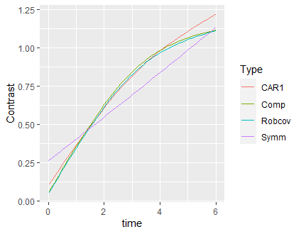
I slightly modified the example, as if my primary analysis question was the – possibly race-dependent – evolution of fbf over time. I hope it is correct in the above way.

(Again, the major point here is that if this robust covariance estimation approach is feasible, then it could be extended totally directly to non-normal responses, such as a binary outcome, which GLS can’t handle.)

2 Likes

This is exceptionally helpful Tamas. You are right the cluster sandwich covariance correction is widely applicable (in terms of types of models) and quick. I’ve done some limited situations with within-subject AR(1)-type correlation and the robust standard error estimate, while not perfect, is acceptable in accuracy. Here are some drawbacks:

  • when using a working independence model as you are doing the cluster sizes are not allowed to vary very much across subjects
  • it works best with a large number of small clusters (just as the cluster bootstrap does)
  • it is very non-robust to dropouts that are not completely random
  • by not having a likelihood function you can’t extend it into a Bayesian framework
  • if subject random effects are very large the estimates of the regression coefficients will be biased just like when omitting an important covariate
1 Like

Thank you Frank @f2harrell very much!

Hi, Dr. Harrell @f2harrell:

In using robcov(), we could use something like, from the “rms” manu,

f ← lrm(y ~ lsp(age,50)*sex, x=TRUE, y=TRUE)
g ← robcov(f, id)

but how about if ids are further nested in say, institutions?

or robcov only accounts for one level, i.e., id?

Thanks.

Only one level. Correlation structure can often be taken care of by clustering on the smallest level but I don’t know about statistical efficiency. Remember that the GEE after-fit covariance matrix correction is a large sample approximate method. When possible it’s better to fully model the correlation structure using a likelihood-based approach.

Hi, Dr. Harrell @f2harrell:

I see. Thanks.

Regarding survival data analysis, then there is another issue: how about if we want interpretation at population level (GEE-type of interpretation) while we have say, ids nested in institutions (or more complex correlation structures)? I think we could do it using “coxme”, but the interpretation is at individual level.

What I could think of is based on Peter Austin’s article (2017). Peter mentioned 3 mixed-effects models. The first is the frailty model, and the other two are:

  1. Piecewise Exponential Survival Models with Mixed Effects

If the hazard function is constant as a function of time, then the exponential survival model and the Poisson regression model can be used interchangeably (Laird & Olivier, 1981). Consequently, the PWE model is equivalent to a Poisson regression model (Rodriguez, 2008; Goldstein, 2011).

  1. Discrete Time Survival Models with Mixed Effects

These models use a discrete version of the hazard function.
Binomial regression models, with a logit, probit or complementary log–log link function can be used to model the probability that the event occurred at a specified discrete time point, conditional on the fact that it had not yet occurred (Rabe-Hesketh & Skrondal, 2012b).

As Peter used “glmer” in “lme4” to run the two models, I think I could use '“geepack” to run the same models to get interpretation at population level. I am not sure, though.

Or all in all, longitudinal survival data analysis has not been developed very well up to now?

References

  1. Peter Austin: A Tutorial on Multilevel Survival Analysis:
    Methods, Models and Applications. International Statistical Review (2017), 85, 2, 185–203 doi:10.1111/insr.12214
1 Like