Short-term mortality prediction with long-term follow-up data

It is well-known that that information should not be discarded during the analysis phase (such as what happens with dichotomization), and one of the typical examples for this point is that if we want to study 30-day mortality, and we know the survival times, we should not use logistic regression (as it would essentially bin the survival times), rather use a Cox-model. And, if doctors insist to see results for the 30-day mark, that’s fine, but then extract it from the Cox-model – it is still no reason to use logistic regression.

The problem I now face is just 30-day mortality prediction, and I indeed have survival times to day precision. But they go to 15 years! Should I apply this advice here as well?! (I.e. use Cox model instead of logistic regression.) While I can’t produce any statistical argument, I very-very much doubt that using information on when the patient died after - say - 10 years has any use for 30-day mortality prediction… But the Cox-model introduces further requirements, chiefly proportionality, which can be avoided with logistic regression.

So, basically my question is: can I still use - in contrast to the general advice - logistic regression in this particular case?

1 Like

I’m sure some other people can formulate this better and correct me if I’m wrong, but the brief answer would be that I think you should just develop a model specifically for the 30-day endpoint and do this using the data/variables that are measured up to the 30 day mark. This refers both to the predictors and the outcome, anyone that is not dead at 30 days was alive and is to be treated as such in this analysis.

Then for some more specifics. Regarding the use of logistic or Cox-models a few things are important. Logistic models try to fit a model for the probability of an outcome and so essentially only consider if a person develops the outcome yes or no. If people are followed over a long period of time however, obviously some people will develop the outcome earlier than others but this information is discarded by the logistic model. In addition, a logistic model in it’s simple form can’t deal with individuals who leave the study due to other reasons (censoring): we don’t know if they develop the outcome or not. Survival models such as the Cox-model model the time-to-event (or time to censoring) and so are specifically suited to dealing with time-to-event data and the censoring issue described above. If your follow-up period is brief (and I think 30 days can be considered short), then these issues are not very prominent and a logistic model can be used for your mortality prediction.

As a second point, on why you should only use data from the first 30 days, if you want to predict short term mortality there will be other variables that are predictive of death than for long term mortality. In the short term, things like acute infection, hospital admission etc will probably predict a higher chance of death as they are indicative of short term (life-)threatening conditions, whereas in the long term predictors related to chronic disease/health such as blood pressure or cholesterol will probably predict mortality as they are indicative of long term health threats such as cardiovascular disease. Take again acute infection as an example, you can die of an acute infection in which case the infection will predict your (short-term) death, but if you live then your long term chance of death will be (almost) unaffected (why would an infection 10 years ago, now predict a substantially higher chance of dying you could ask yourself).

Your post seems to ask if you could use a Cox model with 15 years of data to predict your 30 day mortality. For the reasons above, it (probably) can’t. A Cox model using all 15 years of data is basically a model for predicting long term mortality risk and will probably include measures such as blood pressure. Of course you can ask this model for the predicted mortality at 30 days, but it will likely be 1.) a small probability and 2.) inaccurate because the model (probably) only includes predictors of long term mortality which are not suited/useful for accurate short term predictions.

There are then 2 things you could do. Fit a Cox-model treating everyone who did not die at 30 days as alive at 30 days (so they get censored at the end of the 30 day follow-up). Or, as censoring and time-to-event is less of an issue in such a short time and as you mention Cox-models carry a number of additional assumptions, just fit a logistic model on the 30 day outcome. Set everyone who did not die at the 30 day mark as alive and those that did die as death and use this as the outcome for your model. In both cases, be sure not to include measurements performed after the 30 day mark in your model (not sure about your study design, but in case you have several measurement timepoints for an individual, don’t include data collected after the end of your desired follow-up period. Future data can’t be collected to predict a death in the past in real life practice after all).

6 Likes

I agree with everything in that answer. The one hesitation I have is that someone who dies at 31 days would be treated as a complete success. Instead I’d like to borrow information from them. This could be handled by fitting covariates in the Cox model in the standard way, and adding interactions with all of them and log(time) as time-dependent covariates.

3 Likes

Dear @scboone ,

First of all, thank you very much for your detailed response!

While my question can be considered completely general, two things perhaps worth mentioning that pertain to my concrete problem: 1) I have complete follow-up for all subjects, there is no censoring 2) there are no time-dependent covariates, every explanatory variable represents a measurement made at Time 0.

Your suggestion of censoring everyone after 30 days is absolutely reasonable (and solves my problem, that I didn’t really want deaths after, say, 10 years to have any influence on the result).

Can I summarize your suggestion in the following way: “Using a Cox-regression in the above way will have the advantage of incorporating the information on when the patient died exactly between 0 and 30 (in contrast to logistic regression), at the price of introducing the proportionality assumption”…?

Because this essentially means that we have to weigh these two aspects. If I understand you correctly, your reasoning is that for such a small period, the loss in information is smaller problem than the need for proportionality.

Side note: I personally totally agree, but it’d be interesting to see if there is any way to quantitatively compare them, and judge this.

Finally, the only thing that is unclear, is that this whole logic pertains to smaller follow-up intervals as well, isn’t it. If we have 60 days of follow-up, the textbook advice is very clearly to put them into a Cox model (without any additional censoring!). Why not censor after 30 days in that case as well? Only because of what @f2harrell mentioned, i.e. to borrow data from the time of later deaths too?

1 Like

Good to know, that eases some of the analytical concerns already!

I think this is true as indeed you incorporate time-to-event information. However, the main reason why you can use logistic regression in this context is that there is only a comparatively small variation in time-to-event on such a short interval (effectively it is more or less ignorable, which is what logistic regression does). Because of this, I think there is also little information to gain from just the time-to-event in the 0-30 day interval. However, combined with the suggestion of @f2harrell I think you can use the Cox-model to include additional information from events somewhat into the future.

I think in a sense the suggestion you mention in your last paragraph is sort of a ‘naive’ version of what @f2harrell proposes. If you have 60 days of follow-up and include all this in the model then the follow-up time is still quite short so the estimated model will probably still perform reasonablyl for the short-term 30 day predictions: it is still mostly a model for short term prediction. However the longer this period becomes, the more you are effectively moving towards a long-term risk prediction model. By incorporating the interaction terms with time such as @f2harrell suggests this issue is ameliorated.

1 Like

for what it’s worth, i was just reading this paper which describes their approach in several steps: 30-Day Survival Probabilities as a Quality Indicator for Norwegian Hospitals: Data Management and Analysis

2 Likes

This entire answer is superb, but I have one additional consideration here for the original poster that is as much qualitative as it is quantitative. In some settings, such as intensive care / critical care trials, the choice of a binary outcome (e.g. 30-day or 60-day mortality) rather than time-to-event may actually be preferable, despite the loss of information from the survival times, for reasons explained here.

Briefly, in a critical-care setting, someone might be kept alive for a few extra days by being placed on a ventilator or receiving additional intensive treatments that merely result in a few extra days of suffering; it’s arguable that surviving for 9 days rather than 5 days is not, in fact, a better outcome. Using a time-to-event analysis gives extra benefit to every additional ounce of survival that can be squeezed out of the patient when in reality the question for many ICU trials is “does this treatment increase the chance that this person will leave the hospital alive or not?”

So, while I generally object to the use of logistic regression for any survival outcome where there is any concern at all about censoring, incomplete follow-up, and dislike the loss of information, I definitely can see a reasonable argument for use of a binary “survival to hospital discharge” (or something of that nature) depending on the clinical situation and treatment being studied.

4 Likes

But then I’m worried about the opposite problem. Keeping a patient alive to die on day 31 is considered a total success in a logistic model.

1 Like

What about de-coupling it from time, then, and making it something like “discharged alive” or even “discharged alive to home” (to remove patients that were sent to hospice / skilled nursing facilities because they had not truly recovered, had a stroke, etc) or “discharged alive with good functional capacity” (if that could be defined satisfactorily)?

Furthermore, in an acute setting, the risk of censoring or loss-to-follow-up should be extremely low; I should think they’d be able to determine if the patient died in-hospital vs was discharged alive for all patients.

2 Likes

I like “discharged alive to home”.

First of all, thank you very much for all these excellent ideas and discussions!

I appreciate the paper cited by @ADAlthousePhD , I’ll discuss it with my MD coauthors to see if it applies to our clinical situation.

In the meantime, I am trying to understand the suggestion of @f2harrell and @scboone . I am sorry, I know that these are entirely technical questions, but I don’t have much expertise in this field:

  • To realize this I don’t need to introduce any further censoring, just add the interactions, right?
  • Am I right to assume that these interactions are simply meant to specify time-varying coefficients (i.e. time-varying HRs)…?
  • If so, is my understanding correct that the aim of this is to allow covariates such as infection (in @scboone 's examples) have an effect early on, but this effect will diminish later, and predictors such as blood pressure have little effect initially, but substantially later on? Is this the reason why we need time-varying coefficients?
  • If so, why should we include interaction with log(time)? This seems entirely restrictive to one specific functional form; Frank always emphasizes flexibility, so I don’t really see why shouldn’t we take the interaction with rcs(time). So that the effect in time can indeed be practically any function.

The time-dependent covariates I spoke of were to relax the PH assumption. A spline of t would be even better than log.

Thank you Frank! I know that now this will be a totally technical question, sorry, but… how to do this in rms? I’ve read this guide from Therneau et al, which was really instructive, but it seems to me that cph simply doesn’t support this tt function. Changing the dataset to counting process format also doesn’t work, as we need continuous time for the spline.

1 Like

This should work in rms but I suggest you get it working first in survival::coxph.

I absolutely agree. There is nothing magic about 30 days. In the CCU, surviving 28 days is a good sign, since mortality is concentrated in the early days of admission, but surviving the first year is also a good indicator, because the death rate in the first year is significantly higher than it will subsequently be. So 28-day and 1-year survival make sense.
But with malignancies such as melanoma, the window of early mortality is much larger – years, not days.

The Irish are supposed never to answer a question but instead ask another. So my response would be what’s magic about 30 days?. The investigators should justify their cutoff – and not by saying everyone else did it too. This, as our lawyers advise is, is not a legal defence.

1 Like

Yes, I personally totally agree @RonanConroy . Question is, what other (better) options do we have to characterize “short-term mortality” after a procedure/diagnosis…

There seems to be no downside on doing a Cox regression analysis for the 15 years. You can always calculate the cumulative risk of deaths at any time point from such a model (28, 30, 31 days). The latter is a subject matter issue (i.e. it depends on the problem you are study, not on the method for the analysis). You will get the same estimate of 30 days survival probability if you cut the follow-up time to 30 days or use the 15 years of follow-up. Of course, some risk factors may have a short effect on survival. If you do the Cox regression using the complete follow-up time (15 years) you should check for proportionality. However you should also check for proportionality if you limit the follow-up to 30 days, as this is a key assumption of the Cox model, and the effect of some risk factors could be stronger during the first week of follow-up than later on, for example. If the proportionality assumption is not met for a risk factor, then you may do a Cox regression stratifying for that factor. There are different ways to address the issue of non-proportionality (time-by-factor interactions is one of them).
If you don’t have losses to follow-up (censoring), a logistic regression analysis would give you the same estimates of survival than a Cox model. Of course, it would be unlikely not having losses to follow-up in a 15-year period, but it would be likely if the follow-up is only 30 days. The estimates of the effect of an exposure will be very similar for the logistic and the Cox model. They may be slightly different because the Cox model gives you the rate ratio, while logistic gives you the odds ratio. If the outcome is rare, they would be very close. While doing your logistic model you would still have to consider that some risk factors may have an effect on survival that changes with time. Again, this is a subject matter issue, not a “regression-model” issue. In consequence, you will have to consider an interaction between that risk factor and time. On the other hand, if 30-day risk of death is high (greater than 10%?), logistic will overestimate the effect of some exposures. If that is reason for concern, you may still use logistic, estimate the risk of death from the logistic model, and then calculate the risk ratio based on the estimate risks (i.e. the risk in exposed and non-exposed).
There is little in this comment that have not been included in previous comments. I just tried to focus on your options. IMO, you would be fine with either approach.

OK, then… I finally managed to try out all possible options on a real-life dataset. I’ll now report my findings.

(I used veteran with two modifications: I excluded times after 900 days to limit the time span (those are likely coding errors anyway), and the few censorings to match my – easier – situation in which we have no censored observations).

The explanatory variables were trt, prior and karno. (The Karnofsky-score is continuous, but I put it linearly into the model, yes, of course we should use splines, at least at first, but that’s a separate issue, so for simplicity I omitted it.)

Three possible strategies were outlined in this thread (thanks again especially to @scboone and @f2harrell ):

  • Usual logistic regression, with status at 30 day being the outcome.
  • Usual Cox regression (i.e., proportionality assumption applies) with subjects alive at 30 days artificially censored at 30 days.
  • Cox regression with interaction between each variable and – spline-expanded – time, to allow time-varying coefficients (i.e., proportionality assumption relaxed). In contrast to the previous example, the HR is now not universal, so we have to be careful to extract the HR specifically for 30 days. In this approach we could used the whole timespan without any artificial censoring introduced, but out of curiosity I tried what happens if we censor artificially at X days (X>30). (My rationale for this was that if everything goes well, later and later observations shouldn’t have much impact on the results at 30 days, i.e., this function should converge.)

Here is the script:

library( survival )
library( splines )

data( veteran )

veteran <- veteran[ veteran$time < 900, ] # outliers, likely coding error
veteran <- veteran[ veteran$status==1, ] # to simulate my (easier) situation when
# we have no censoring

vettimes <- sort( unique( veteran$time ) )

# 1st approach: logistic regression

fit1 <- glm( I(veteran$time<=30) ~ trt + prior + karno, data = veteran )
summary( fit1 )
coef( fit1 )[ "karno" ]

# 2nd approach: censor everyone (artificially) at 30 days, and run a usual
# Cox-regression (i.e. proportionality assumption applies)

veteran$status2 <- ifelse( veteran$time<30, 1, 0 )
veteran$time2 <- ifelse( veteran$time<30, veteran$time, 30 )
fit2 <- coxph( Surv( time2, status2 ) ~ trt + prior + karno, data = veteran )
summary( fit2 )
coef( fit2 )[ "karno" ]

# 3rd approach: censor everyone (artificially) at X days (x>30), and run a
# Cox-regression with interaction with time (i.e. proportionality assumption
# relaxed).

fit3s <- lapply( vettimes[ vettimes>30 ], function( t ) {
  veteran$status2 <- ifelse( veteran$time<t, 1, 0 )
  veteran$time2 <- ifelse( veteran$time<t, veteran$time, t )
  veteran3 <- survSplit( Surv( time2, status2 ) ~ trt + prior + karno,
                         data = veteran, cut = 1:max( veteran$time ) )
  coxph( Surv( tstart, time2, status2 ) ~ trt + trt:ns( time2, df = 4 ) +
           prior + prior:ns( time2, df = 4 ) +
           karno + karno:ns( time2, df = 4 ), data = veteran3 )
})

coeffit3karno <- sapply( fit3s, function( f )
  eval( attr( terms( f ), "predvars" )[[ 4 ]],
        data.frame(time2 = 30) ) %*% coef(f)[ grep( "karno.*time2|time2.*karno",
                                                    names( coef( f ) ) ) ] +
    coef( f )[ "karno" ] )

# Comparing the three approaches

plot( vettimes[ vettimes>30 ], coeffit3karno,
      type = "l", ylim = c( -0.07, 0.02 ), ylab = "OR/HR/HR@30days",
      xlab = "Artificial censor time [days]" )
abline( h = coef( fit1 )[ "karno" ], col = "blue" )
abline( h = coef( fit2 )[ "karno" ], col = "red" )

And the result:

Rplot36

First of all, we see that the third approach’s value indeed converges. Interestingly, the values with the second and the third approach were quite similar (don’t forget that the “result from the third approach” means the end of the black line). The result of the logistic regression, however, is quite different.

I hope I correctly understood and implemented every idea, but nevertheless, I’d appreciate if you’d check the code, and I of course welcome any further remark or criticism.

2 Likes

Thanks for taking the time to report back with your attempts and for illustrating them with a build-in dataset! I think your code looks good, but I am not very experienced in the use of splines myself so I hope someone else can check the code for method 3. The convergence of method 2 and 3 (at the end with basically no censoring) looks nice and this is a very nice graphical illustration to see this.

You mention the results are quite different for the logistic regression, but maybe the difference is not so extreme as you think. To start the values you report now are not the OR and HR, rather they are the ln(OR) and ln(HR) as you are directly plotting the coefficients from the modelling steps in R. R by default reports the coefficients on the scale on which the models are fitted, which is the log-scale for both logistic and the Cox-model.

The log(OR) is roughly -0.013 while the ln(HR) from method 2 is -0.056. Translated into the respective OR and HR this is:

exp(-0.013) = 0.987
exp(-0.056) = 0.946

So true, there seems to be some difference, however I think there is a good chance this is explained by the differences in the methods in which a Cox- and logistic model are constructed (Cox still incorporates the time to event for these 30 days). Add to this the fact that the OR/HR per point Karnofsky score is not that large, while you also have a small number of cases in the first 30 days:

sum(veteran$time<30)
[1] 40

You only have 40 cases in this short time period, while fitting a model with 3 variables, which I think also probably leads to some instability in your estimates?

Below is the graph with the OR/HR after transformation!

Thanks @scboone for the detailed reply!

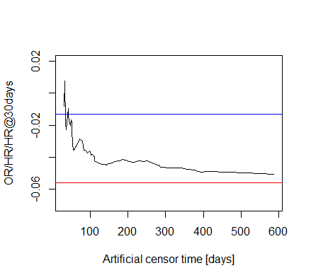
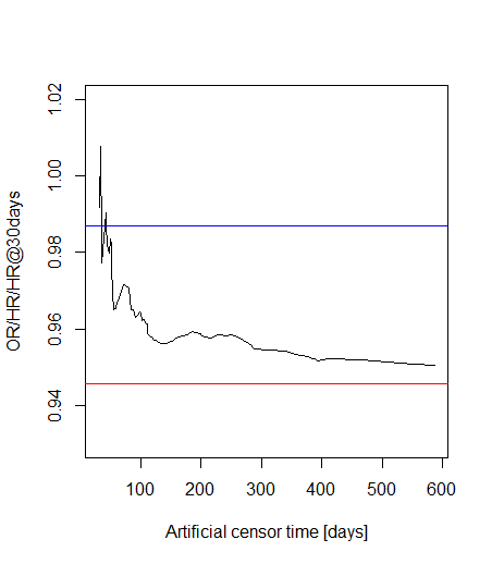
The fact that method 3 converges to something with increasing X is indeed nice, however, that method 2 and 3 converges to each other is not trivial (at least in my understanding!) as one represents a Cox regression with proportionality assumption, but it is relaxed in the other.

Ah, of course, sorry. I don’t want to introduce further transformations, but the vertical axis should indeed be relabeled.

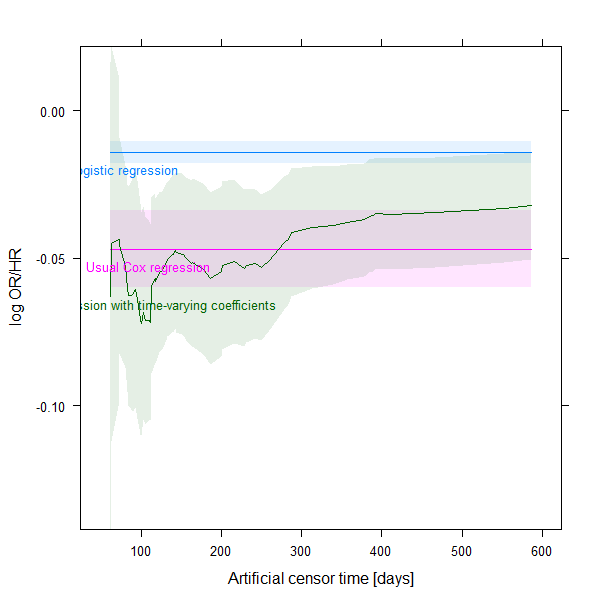
There is another way to look this, and I really just forget to do it originally: we could also have a look at the confidence intervals! My updated code below will do this. (But I am not 100% sure in how to calculate the CI for the spline, hope this is correct…)

That’s right, perhaps the example is not the best from this aspect.

Well, we have 39 deaths for 3 covariates, that doesn’t seem horribly bad, but I now increased the cut-off time to 60 days, so we surely have plenty of events.

Updated code:

library( survival )
library( splines )

data( veteran )

veteran <- veteran[ veteran$time < 900, ] # outliers, likely coding error
veteran <- veteran[ veteran$status==1, ] # to simulate my (easier) situation when
# we have no censoring

vettimes <- sort( unique( veteran$time ) )

CutoffDay <- 60

# 1st approach: logistic regression

fit1 <- glm( I(veteran$time<=CutoffDay) ~ trt + prior + karno, data = veteran )
summary( fit1 )
coeffit1karno <- data.frame( times = vettimes[ vettimes>CutoffDay ],
                             approach = "Logistic regression",
                             coef = coef( fit1 )[ "karno" ],
                             t( confint( fit1 )[ "karno", ] ),
                             row.names = NULL )

# 2nd approach: censor everyone (artificially) at 30 days, and run a usual
# Cox-regression (i.e. proportionality assumption applies)

veteran$status2 <- ifelse( veteran$time<CutoffDay, 1, 0 )
veteran$time2 <- ifelse( veteran$time<CutoffDay, veteran$time, CutoffDay )
fit2 <- coxph( Surv( time2, status2 ) ~ trt + prior + karno, data = veteran )
summary( fit2 )
coeffit2karno <- data.frame( times = vettimes[ vettimes>CutoffDay ],
                             approach = "Usual Cox regression",
                             coef = coef( fit2 )[ "karno" ],
                             t( confint( fit2 )[ "karno", ] ),
                             row.names = NULL )

# 3rd approach: censor everyone (artificially) at X days (x>30), and run a
# Cox-regression with interaction with time (i.e. proportionality assumption
# relaxed).

fit3s <- lapply( vettimes[ vettimes>CutoffDay ], function( t ) {
  veteran$status2 <- ifelse( veteran$time<t, 1, 0 )
  veteran$time2 <- ifelse( veteran$time<t, veteran$time, t )
  veteran3 <- survSplit( Surv( time2, status2 ) ~ trt + prior + karno,
                         data = veteran, cut = 1:max( veteran$time ) )
  coxph( Surv( tstart, time2, status2 ) ~ trt + trt:ns( time2, df = 4 ) +
           prior + prior:ns( time2, df = 4 ) +
           karno + karno:ns( time2, df = 4 ), data = veteran3 )
})

coeffit3karno <- do.call( rbind, lapply( fit3s, function( f ) {
  SplineMat <- cbind( 1, eval( attr( terms( f ), "predvars" )[[ 4 ]],
                               data.frame( time2 = CutoffDay ) ) )
  sel <- grep( "karno", names( coef( f ) ) )
  se <- sqrt( diag( SplineMat%*%vcov( f )[ sel, sel ]%*%t(SplineMat) ) )
  data.frame( approach = "Cox regression with time-varying coefficients",
              coef = SplineMat%*%coef( f )[ sel ],
              X2.5.. = SplineMat%*%coef( f )[ sel ] + qnorm( 0.025 )*se,
              X97.5.. = SplineMat%*%coef( f )[ sel ] + qnorm( 0.975 )*se )
} ) )

# Comparing the three approaches

coeffitskarno <- rbind( coeffit1karno, coeffit2karno, 
                        data.frame( times = vettimes[ vettimes>CutoffDay ],
                                    coeffit3karno ) )

Hmisc::xYplot(Hmisc::Cbind( coef, X2.5.., X97.5.. ) ~ times,
              groups = approach, data = coeffitskarno, type = "l",
              ylab = "log OR/HR", xlab = "Artificial censor time [days]",
              method = "filled bands",
              col.fill=scales::alpha(lattice::trellis.par.get()$superpose.line$col,
                                     0.1 ) )

And the results:

2 Likes