I am comparing two diagnostic methods, Method 1 and Method 2, where Method 2 is considered the gold standard. I am using Method 1 to predict the Method 2 using logistic regression. My dataset contains approximatelly 5,000 datapoints.
I encountered an issue with the intercepts of specific probabilities between two implementations of logistic regression: R’s glm function and Python’s scikit-learn.
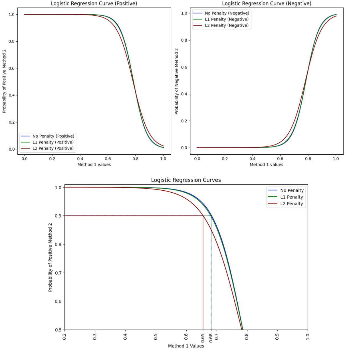
R’s glm doesn’t apply regularization by default, whereas Python Scikit-Learn LogisticRegression() uses L2 regularization by default.
To illustrate, here is my Python code:
import numpy as np
import pandas as pd
import matplotlib.pyplot as plt
from sklearn.linear_model import LogisticRegression

# Hyperparemeters
THRESHOLD = 0.80
DIAG_ACCURACY = 0.90

file_path = r"datasheet.xlsx"
data = pd.read_excel(file_path)

data['method_2_positive'] = (data['method_2'] < THRESHOLD).astype(int)

X = data[['method_1']]
y_pos = data['method_2_positive']

# Model training without penalty
model_none = LogisticRegression(penalty=None, solver='lbfgs').fit(X.values, y_pos)

# Model training with L1 penalty
model_l1 = LogisticRegression(penalty='l1', solver='liblinear').fit(X.values, y_pos)

# Model training with L2 penalty (default in Scikit-learn)
model_l2 = LogisticRegression(penalty='l2', solver='lbfgs').fit(X.values, y_pos)

# Range of values to predict
X_pred = np.linspace(X.values.min(), X.values.max(), 300).reshape(-1, 1)

# Curves for model without penalty
prob_pos_none = model_none.predict_proba(X_pred)[:, 1]  # Probability of positive
prob_neg_none = model_none.predict_proba(X_pred)[:, 0]  # Probability of negative

# Curves for model with L1 penalty
prob_pos_l1 = model_l1.predict_proba(X_pred)[:, 1]  # Probability of positive
prob_neg_l1 = model_l1.predict_proba(X_pred)[:, 0]  # Probability of negative

# Curves for model with L2 penalty
prob_pos_l2 = model_l2.predict_proba(X_pred)[:, 1]  # Probability of positive
prob_neg_l2 = model_l2.predict_proba(X_pred)[:, 0]  # Probability of negative

# Plotting the logistic regression curves
plt.figure(figsize=(12, 6))

plt.subplot(1, 2, 1)
plt.plot(X_pred, prob_pos_none, label='No Penalty (Positive)', linestyle='-', color='blue')
plt.plot(X_pred, prob_pos_l1, label='L1 Penalty (Positive)', linestyle='-', color='green')
plt.plot(X_pred, prob_pos_l2, label='L2 Penalty (Positive)', linestyle='-', color='darkred')
plt.xlabel('Method 1 values')
plt.ylabel('Probability of Positive Method 2')
plt.title('Logistic Regression Curve (Positive)')
plt.legend()

plt.subplot(1, 2, 2)
plt.plot(X_pred, np.abs(1-prob_pos_none), label='No Penalty (Negative)', linestyle='-', color='blue')
plt.plot(X_pred, np.abs(1-prob_pos_l1), label='L1 Penalty (Negative)', linestyle='-', color='green')
plt.plot(X_pred, np.abs(1-prob_pos_l2), label='L2 Penalty (Negative)', linestyle='-', color='darkred')
plt.xlabel('Method 1 values')
plt.ylabel('Probability of Negative Method 2')
plt.title('Logistic Regression Curve (Negative)')
plt.legend()
plt.tight_layout()
plt.show()

# Intercepts at 90% probability
positive_intercept_none = X_pred[np.abs(prob_pos_none - DIAG_ACCURACY).argmin()]
positive_intercept_l1 = X_pred[np.abs(prob_pos_l1 - DIAG_ACCURACY).argmin()]
positive_intercept_l2 = X_pred[np.abs(prob_pos_l2 - DIAG_ACCURACY).argmin()]

print(f'''
Positive Intercept (No Penalty): {positive_intercept_none[0]:.2f}
Positive Intercept (L1 Penalty): {positive_intercept_l1[0]:.2f}
Positive Intercept (L2 Penalty): {positive_intercept_l2[0]:.2f}
''')

# Zoom plot
plt.figure(figsize=(10,6))

# No Penalty
plt.plot(X_pred, prob_pos_none, label='No Penalty', linestyle='-', color='blue')
plt.hlines(DIAG_ACCURACY, X_pred.min(), positive_intercept_none, linestyle=':', color='blue', linewidth=1)
plt.vlines(positive_intercept_none, 0.5, DIAG_ACCURACY, linestyle=':', color='blue', linewidth=1)


# L1 Penalty
plt.plot(X_pred, prob_pos_l1, label='L1 Penalty', linestyle='-', color='green')
plt.hlines(DIAG_ACCURACY, X_pred.min(), positive_intercept_l1, linestyle='-', color='green', linewidth=1, alpha=0.5)
plt.vlines(positive_intercept_l1, 0.4, DIAG_ACCURACY, linestyle='-', color='green', linewidth=1, alpha=0.5)

# L2 Penalty
plt.plot(X_pred, prob_pos_l2, label='L2 Penalty', linestyle='-', color='darkred')
plt.hlines(DIAG_ACCURACY, X_pred.min(), positive_intercept_l2, linestyle='-', color='darkred', linewidth=1)
plt.vlines(positive_intercept_l2, 0.4, DIAG_ACCURACY, linestyle='-', color='darkred', linewidth=1)

# Plot configuration
plt.xlabel('Method 1 Values')
plt.ylabel('Probability of Positive Method 2')
plt.title('Logistic Regression Curves')
plt.xlim(0.2, 1.0)
plt.ylim(0.5, 1.01)

plt.xticks(ticks=np.append(plt.xticks()[0], [positive_intercept_l2, positive_intercept_none]),
           labels=np.append(plt.xticks()[1], [f'{positive_intercept_l2[0]:.2f}', f'{positive_intercept_none[0]:.2f}']))
plt.xticks(rotation=90)

plt.legend()
Given this context, my question is:
Should I use regularization (L1 or L2) for univariate logistic regression in this diagnostic comparison? If yes, which regularization technique is recommended and why?
I am looking for insights on whether regularization is necessary in this case and how it impacts the model’s performance and interpretability, since it changes considerably the curves.
Thank you in advance for your help!