I’m currently working on an informal simulation study to show the dangers of dichotomizing a continuous variable. I’ve been working a lot lately with genetic and molecular prognostic markers, and the literature is filled with studies that divide patients into low expression and high expression groups and then compare their survival differences. I’ve encountered many researchers that seem to think this is the proper way to analyze continuous variables, justified in part because so many papers dichotomize.
The goal of the simulation study is to demonstrate that using continuous methods (Cox regression) have higher statistical power than dichotomous methods (dichotomized Kaplan Meier analysis). I simulate data from an exponential distribution using formula derived by Bender et al. and code from an example in 18.3.3 in the BBR notes. The variable of interest is a continuous covariate generated from a standard normal distribution that linearly affects the hazard function. My results for data simulated with \lambda_0=.05 and maximum time of 30 months are shown below
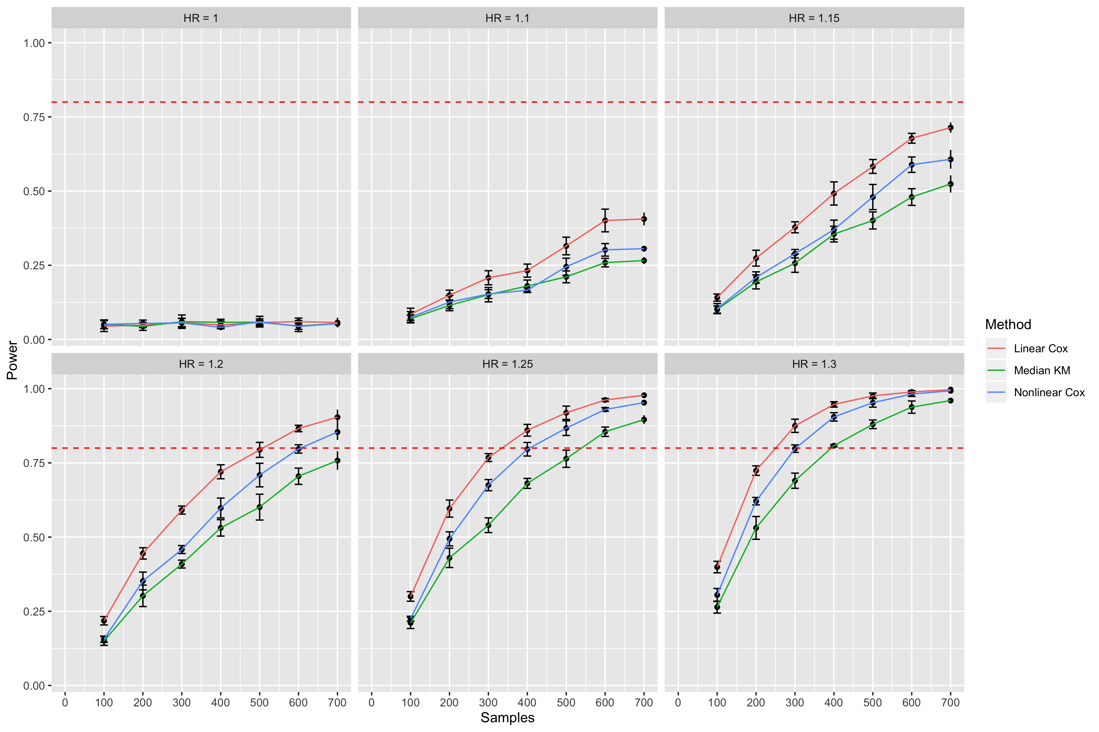
Figure 1. Statistical power calculation comparing median cutpoint Kaplan Meier analysis (Median KM) with linear and nonlinear Cox regression. Error bars are 95% confidence intervals. Dashed red line represents 80% power. HR=Hazard Ratio.
For each N and hazard ratio combination, I simulated datasets from 5 different seeds to quantify the uncertainty surrounding the data generating seed that is chosen. For each seed, I generated 200 datasets, fit models to each dataset (median cutpoint-log rank test, linear and nonlinear Cox regressions) and computed the power of each model for that seed. Using \alpha=.05, power was calculated by counting the number of datasets where p<.05 and dividing by 200 (the total number of datasets for that seed). This yielded 5 point estimates of power, allowing me to compute 95% confidence intervals (error bars on the graph). The median was used for the dichotomous model, and a restricted cubic spline with 3 knots from the rcs function in rms was used for the nonlinear Cox model.
Although my results recapitulate the statistical literature that states continuous methods will have more power than dichotomous methods, I was surprised by the relatively poor performance of the nonlinear model compared to the linear model. The poor performance doesn’t really make sense to me, as Harrell states in Regression Modeling Strategies Section 2.4
A better approach that maximizes power and that only assumes a smooth relationship is to use regression splines for predictors that are not known to predict linearly.
Is the nonlinear Cox model performing poorly because the continuous covariate is linearly related to survival? If the true relationship is linear, should we expect subpar power from a nonlinear model? Is my simulation flawed, and we actually expect the nonlinear Cox model to have equivalent power to the linear Cox model? In the field it often makes more sense to assume less and just treat continuous variables as nonlinear, but I’m curious if we could actually be harming our study by using a nonlinear method when the true relationship is linear. I’m also interested to hear thoughts on whether I should be using a more complex distribution like Weibull or Gompertz.
Here’s my code:
# File: simulations.R
library(survival)
library(dplyr)
library(tidyr)
library(ggplot2)
library(forcats)
library(rms)

simulate_data <- function(N, maxtime, beta, baseline_hazard, seed) {
  # See Bender et al. 2005 for more information on parametric survival simulation
  # Assume continuous covariate follows a standard normal distribution
  covariate_mean <- 0
  covariate_sd <- 1
  covariate <- rnorm(N, covariate_mean, covariate_sd) # create covariate
  cens <- maxtime * runif(N) # create censoring times (unrelated to survival)
  h <- baseline_hazard * exp(beta * (covariate - covariate_mean))
  dt <- -log(runif(N)) / h # Bender formula for times T ~ Exponential(baseline_hazard)
  e <- ifelse(dt <= cens, 1, 0)
  dt <- pmin(dt, cens)
  S <- Surv(dt, e)
  linear.fit <- coxph(S ~ covariate)
  median.fit <- coxph(S ~ covariate > median(covariate))
  nonlinear.fit <- cph(S ~ rcs(covariate, 3))
  linear.pvalue <- coef(summary(linear.fit))[, 5]
  median.pvalue <- coef(summary(median.fit))[, 5]
  nonlinear.pvalue <- anova(nonlinear.fit)['covariate', 'P']
  c(linear = linear.pvalue,
    median = median.pvalue,
    nonlinear = nonlinear.pvalue,
    samples = N,
    beta = beta,
    seed = seed)
}

simulate_trial <- function(n_sim, N, maxtime, beta, baseline, seed) {
  set.seed(seed)
  results <- replicate(n_sim, simulate_data(N, maxtime, beta, baseline, seed))
  data.frame(t(results))
}

build_design_matrix <- function(initial_seed, num_seeds, sample_sizes, betas) {
  set.seed(initial_seed)
  seeds <- sample.int(100000, num_seeds)
  design <- expand.grid(
    N = sample_sizes,
    logHR = betas,
    seed = seeds
  )
}

compute_power <- function(simulation_results) {
  power_info <- simulation_results %>%
    gather("linear", "median", "nonlinear",
           key="model", value="pvalue") %>%
    mutate(model = factor(model)) %>%
    mutate(model = fct_recode(model,
                              `Linear Cox` = "linear",
                              `Median KM` = "median",
                              `Nonlinear Cox` = "nonlinear"
                              )) %>%
    group_by(model, samples, beta, seed) %>%
    summarise(power = sum(pvalue < .05) / n()) %>%
    group_by(model, samples, beta) %>%
    summarise(mean_power = mean(power),
              se = sd(power) / sqrt(n()),
              lower = mean_power - se,
              upper = mean_power + se,
              lower_ci = mean_power - 1.96 * se,
              upper_ci = mean_power + 1.96 * se) %>%
    mutate(HR = paste("HR =", exp(beta)))
}

plot_results <- function(power_results) {
  # Plots 95% confidence intervals, NOT standard error
  power_plot <- power_results %>%
    ggplot(aes(samples, mean_power)) +
    geom_point() +
    geom_errorbar(aes(ymin = lower_ci, ymax = upper_ci), width=20) +
    geom_line(aes(color = factor(model))) +
    facet_wrap(~HR) +
    geom_hline(yintercept = .8, color="red", linetype="dashed") +
    labs(x = "Samples", y = "Power") +
    guides(color=guide_legend(title="Method")) +
    scale_x_continuous("Samples", breaks=seq(0, 700, by=100), limits=c(0, 700))
}

run_simulation <- function(save_figure=F) {
  n_sims <- 200
  maxtime <- 30
  baseline <- .05

  sample_sizes <- c(100, 200, 300, 400, 500, 600, 700)
  betas <- log(c(1.0, 1.1, 1.15, 1.2, 1.25, 1.3))
  setup_seed <- 42
  n_seeds <- 5

  design <- build_design_matrix(setup_seed, n_seeds, sample_sizes, betas)
  results <- design %>%
    rowwise() %>%
    do(simulate_trial(n_sims, .$N, maxtime, .$logHR, baseline, .$seed))
  power_results <- compute_power(results)
  power_plot <- plot_results(power_results)
  print(power_plot)
  if(save_figure) {
    ggsave(file.path(getwd(), "power_plot.png"), width = 12, height = 8)
  }
}

run_simulation(save_figure=T)