Stratifying by year of treatment in observational studies

albertoca · October 7, 2019, 5:07pm

Another quick doubt, this is the result of anova(fit) from a Cox model with interactions.
I have used a non-linear interaction between the effect of treatment and year.
How should I interpret and report these pvalues?
Is it significant or not?

treat * year (Factor+Higher Order Factors) 5.42 2 0.0665
Nonlinear 4.70 1 0.0301
Nonlinear Interaction : f(A,B) vs. AB 4.70 1 0.0301

f2harrell · October 7, 2019, 6:29pm

You have mild evidence against the presupposition that the treatment effect is constant over time. But rely on confidence intervals no matter what the p-value. Type ?contrast.rms to see examples of how to plot the treatment effect over time using the rms package contrast function. This will look something like:

yrs <- seq(1990, 2019, length=150)
k <- contrast(fit, list(treatment='b', year=yrs),
                   list(treatment='a', year=yrs))

which computes hazard ratios as a function of year.

albertoca · October 7, 2019, 7:08pm

Yes, I’ve already seen that the contrast function is fabulous. That’s what I like most about rms (also splines). Together with ggplot you can draw very cool graphics. But don’t you like interaction tests in general or just applied to continuous variables such as year? Do you think it makes sense to include them together with contrasts or not?

f2harrell · October 7, 2019, 8:03pm

I’m not understanding the new question.

albertoca · October 7, 2019, 8:40pm

Sorry, the question is whether you have general objections to interaction tests to evaluate whether the hazard ratio of a therapeutic effect along two levels of a factor is similar or not. For example, right now it appears to me that the effect of DCF in intestinal tumors has hazard ratio 0.80, in diffuse 0.91. The interaction test (associated to the term treat*histology) is not significant. In this case, I also have to rely only on the confidence intervals, or the interaction tests do have value here.

f2harrell · October 8, 2019, 12:45pm

It’s actually a tricky question because the power of interaction tests is low. We tend to trust interaction tests only when they are “significant” which creates a selection/publication bias. The Bayesian approach of the interaction “half in and half out of the model” is much needed. In the frequentist paradigm I would focus on confidence bands for interaction effects (double differences). In your case the interaction test does have a little indirect value—you’re able to say that with the present information/sample size you were unable to contradict the supposition of constant treatment effect.

albertoca · October 8, 2019, 5:54pm

I apologize in advance to Professor Harrell for my enthusiasm.
I have made my first attempt at Bayesian subgroup analysis and I think it is precious, but let’s see if it is correct.
According to a meta-analysis, the effect of docetaxel on OS is: HR 0.86 (95% CI 0.78 to 0.95).

ncbi.nlm.nih.gov

Chemotherapy for advanced gastric cancer.

AD Wagner, NL Syn, M Moehler, W Grothe, WP Yong, BC Tai, J Ho and S Unverzagt, The Cochrane database of systematic reviews, 29 2017 08

Gastric cancer is the fifth most common cancer worldwide. In "Western" countries, most people are either diagnosed at an advanced stage, or develop a relapse after surgery with curative intent. In people with advanced disease, significant benefits from targeted therapies are currently limited to HER-2 positive disease treated with trastuzumab, in combination with chemotherapy, in first-line. In second-line, ramucirumab, alone or in combination with paclitaxel, demonstrated significant survival benefits. Thus, systemic chemotherapy remains the mainstay of treatment for advanced gastric cancer. Uncertainty remains regarding the choice of the regimen.To assess the efficacy of chemotherapy versus best supportive care (BSC), combination versus single-agent chemotherapy and different chemotherapy combinations in advanced gastric cancer.We searched the Cochrane Central Register of Controlled Trials, MEDLINE and Embase up to June 2016, reference lists of studies, and contacted pharmaceutical companies and experts to identify randomised controlled trials (RCTs).We considered only RCTs on systemic, intravenous or oral chemotherapy versus BSC, combination versus single-agent chemotherapy and different chemotherapy regimens in advanced gastric cancer.Two review authors independently identified studies and extracted data. A third investigator was consulted in case of disagreements. We contacted study authors to obtain missing information.We included 64 RCTs, of which 60 RCTs (11,698 participants) provided data for the meta-analysis of overall survival. We found chemotherapy extends overall survival (OS) by approximately 6.7 months more than BSC (hazard ratio (HR) 0.3, 95% confidence intervals (CI) 0.24 to 0.55, 184 participants, three studies, moderate-quality evidence). Combination chemotherapy extends OS slightly (by an additional month) versus single-agent chemotherapy (HR 0.84, 95% CI 0.79 to 0.89, 4447 participants, 23 studies, moderate-quality evidence), which is partly counterbalanced by increased toxicity. The benefit of epirubicin in three-drug combinations, in which cisplatin is replaced by oxaliplatin and 5-FU is replaced by capecitabine is unknown.Irinotecan extends OS slightly (by an additional 1.6 months) versus non-irinotecan-containing regimens (HR 0.87, 95% CI 0.80 to 0.95, 2135 participants, 10 studies, high-quality evidence).Docetaxel extends OS slightly (just over one month) compared to non-docetaxel-containing regimens (HR 0.86, 95% CI 0.78 to 0.95, 2001 participants, eight studies, high-quality evidence). However, due to subgroup analyses, we are uncertain whether docetaxel-containing combinations (docetaxel added to a single-agent or two-drug combination) extends OS due to moderate-quality evidence (HR 0.80, 95% CI 0.71 to 0.91, 1466 participants, four studies, moderate-quality evidence). When another chemotherapy was replaced by docetaxel, there is probably little or no difference in OS (HR 1.05; 0.87 to 1.27, 479 participants, three studies, moderate-quality evidence). We found there is probably little or no difference in OS when comparing capecitabine versus 5-FU-containing regimens (HR 0.94, 95% CI 0.79 to 1.11, 732 participants, five studies, moderate-quality evidence) .Oxaliplatin may extend (by less than one month) OS versus cisplatin-containing regimens (HR 0.81, 95% CI 0.67 to 0.98, 1105 participants, five studies, low-quality evidence). We are uncertain whether taxane-platinum combinations with (versus without) fluoropyrimidines extend OS due to very low-quality evidence (HR 0.86, 95% CI 0.71 to 1.06, 482 participants, three studies, very low-quality evidence). S-1 regimens improve OS slightly (by less than an additional month) versus 5-FU-containing regimens (HR 0.91, 95% CI 0.83 to 1.00, 1793 participants, four studies, high-quality evidence), however since S-1 is used in different doses and schedules between Asian and non-Asian population, the applicability of this finding to individual populations is uncertain.Chemotherapy improves survival (by an additional 6.7 months) in comparison to BSC, and combination chemotherapy improves survival (by an additional month) compared to single-agent 5-FU. Testing all patients for HER-2 status may help to identify patients with HER-2-positive tumours, for whom, in the absence of contraindications, trastuzumab in combination with capecitabine or 5-FU in combination with cisplatin has been shown to be beneficial. For HER-2 negative people, all different two-and three-drug combinations including irinotecan, docetaxel, oxaliplatin or oral 5-FU prodrugs are valid treatment options for advanced gastric cancer, and consideration of the side effects of each regimen is essential in the treatment decision. Irinotecan-containing combinations and docetaxel-containing combinations (in which docetaxel was added to a single-agent or two-drug (platinum/5-FUcombination) show significant survival benefits in the comparisons studied above. Furthermore, docetaxel-containing three-drug regimens have increased response rates, but the advantages of the docetaxel-containing three-drug combinations (DCF, FLO-T) are counterbalanced by increased toxicity. Additionally, oxaliplatin-containing regimens demonstrated a benefit in OS as compared to the same regimen containing cisplatin, and there is a modest survival improvement of S-1 compared to 5-FU-containing regimens.Whether the survival benefit for three-drug combinations including cisplatin, 5-FU, and epirubicin as compared to the same regimen without epirubicin is still valid when second-line therapy is routinely administered and when cisplatin is replaced by oxaliplatin and 5-FU by capecitabine is questionable. Furthermore, the magnitude of the observed survival benefits for the three-drug regimens is not large enough to be clinically meaningful as defined recently by the American Society for Clinical Oncology (Ellis 2014). In contrast to the comparisons in which a survival benefit was observed by adding a third drug to a two-drug regimen at the cost of increased toxicity, the comparison of regimens in which another chemotherapy was replaced by irinotecan was associated with a survival benefit (of borderline statistical significance), but without increased toxicity. For this reason irinotecan/5-FU-containing combinations are an attractive option for first-line treatment. Although they need to be interpreted with caution, subgroup analyses of one study suggest that elderly people have a greater benefit form oxaliplatin, as compared to cisplatin-based regimens, and that people with locally advanced disease or younger than 65 years might benefit more from a three-drug regimen including 5-FU, docetaxel, and oxaliplatin as compared to a two-drug combination of 5-FU and oxaliplatin, a hypothesis that needs further confirmation. For people with good performance status, the benefit of second-line chemotherapy has been established in several RCTs.

In our observational study, we found HR 0.84 (95% CI, 0.71-0.99).
However, no one has evaluated the effect in subgroups defined according to histology, and they are really different pathologies that do not have to respond the same. This is of great clinical importance because we are talking about a very toxic therapy, which perhaps not everyone requires.
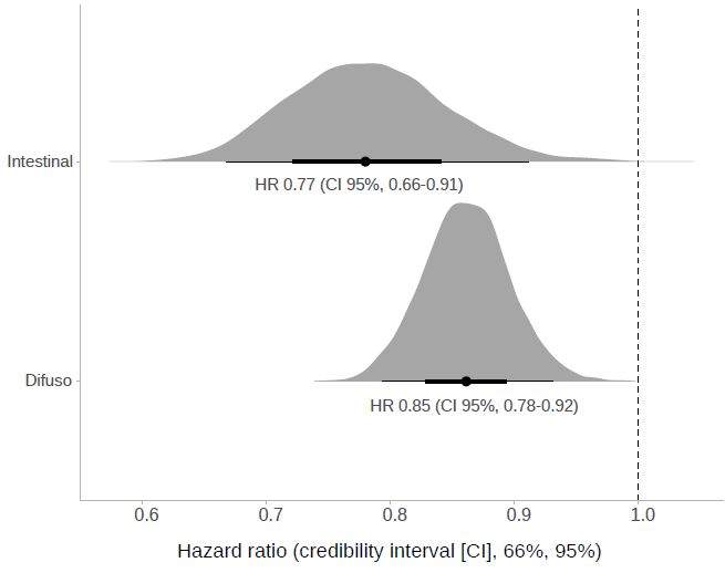
When we evaluate the effect in intestinal histology we get a HR of 0.68 (95% CI, 0.51-0.90), compared to HR of 0.89 (95% CI, 0.91-1.09) in diffuse subtype. However, the interaction test is not significant, p=0.13.
I suppose the usual thing would be to recognize that we have no evidence to say that the therapeutic effect is different in each pathology.
What does Bayesian analysis suggest in this case?
What I have done is feed the model with the prior of Wagner’s meta-analysis assuming that the effect is similar in both subgroups, and I have used a weakly informative prior for the interaction, allowing for some changes. The intervals I get are very similar to the previous ones.
However, what comes out is that the posterior probability of a clinically substantial result (e.g., increase OS >30%) is 70% for the intestinal subtype, but only 6% for the diffuse subtype. When I analyze the posterior probability density for the term treatment*histology interaction, only 19% of the probability mass is within the ROPE, then most likely there is an interaction after all.
Graphs are also awesome.
Is this reasonable?

f2harrell · October 8, 2019, 6:02pm

I hope someone will answer this. In the meantime, if the observational study has a bias in estimating an overall treatment effect, it will not be able to estimate covariate-specific treatment effects.

albertoca · October 8, 2019, 6:05pm

That’s what I get for writing too long. I’m sorry for importuning… There doesn’t seem to be any bias. Our result is similar to the available meta-analysis (HR 0.84 vs 0.86).

albertoca · October 9, 2019, 3:15pm

But, a quick, total neophyte doubt about Bayesian interaction terms. Imagine that I make a Bayesian survival model such as: OS ~ a + a*b, where a and b are two dummie variables that can be 0 or 1.
I want to interpret the coefficient of a*b with a Bayesian approach.
Is it a good practice to use the posterior probability density for the coefficient of a*b to decide if there is substantial interaction? For example, could I evaluate the probability that the coefficient is outside the region of practical equivalence (ROPE 0+/- 10%) and decide on the subgroup effect according to this criterion? Thanks.

f2harrell · October 9, 2019, 11:04pm

You can compute the posterior probability that the absolute value of the interaction parameter exceeds some threshold. Or just make the right covariate-dependent treatment contrasts whether the interaction is impressive or not, since you have already committed to putting the interaction term in the Bayesian model.

albertoca · October 13, 2019, 2:06pm

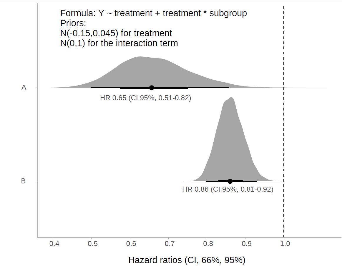
I think one relevant aspect is that there are many subtleties in the choice of priors with interactions. For example, if I use an informative prior for a, for example N(-0.15,0,045) and a weakly informative prior for the interaction a*b, such as N(0,1), the problem is that I am not assuming the same prior for a as a function of each of the b levels.
This could condition the result if 1-a is evaluated instead of a. The question would be what priors do I have to use for interaction terms to assume that both levels of a are under the same prior?

f2harrell · October 13, 2019, 5:13pm

I would think of this as what prior represents the range and relative probabilities of differential treatment effects. The interaction prior induces a correlation between the knowledge of x-specific treatment effects where x is the interacting factor. I would tend to use a skeptical prior for the treatment effect in the reference level of x, and an even more skeptical prior for the double differences.

albertoca · October 13, 2019, 7:28pm

Thank you, Frank.
In the photo what I got so far…

The formula is simplified, the model is much more complex.
For the interaction I used what Andrew Gelman calls in his blog a generic weakly informative prior: normal(0, 1)…
You now suggest that I should use a prior more skeptical than normal (0,1) for the interaction term.
I think it would be reasonable to consider normal (0,0.1). On the other hand, an even more skeptical prior, such as normal (0,0.05) might suppose to assume too much, for example, to assume that I already know that the modification of the effect is going to be very tiny, when in fact this is not clear.
Isn’t it a little subjective? How do I defend normal(0,0.1) against any other option? Does that seem reasonable to you?

f2harrell · October 14, 2019, 2:16pm

I like your way of thinking. I would just change the metric for choosing the prior from variance to the probability that the differential effect exceeds some meaningful level, and solve for the variance that gives you that probability.

albertoca · October 14, 2019, 9:31pm

I’ve been trying that. What I thought was to use the meta-analysis main effect estimate as prior when the interaction was null. Then I did what you said, selecting the prior for the interaction term based on plausible values from previous individual studies within the meta-analysis rather than variance. The result better reflects previous knowledge. However, I have realized how important it is to be rigorous, not only in the choice of prior, as it conditions the outcome, but in the interpretation of posterior bayesian results, which are largely due to our decisions. Notice the change with the previous result.