Stratifying by year of treatment may suppose two relevant aspects to consider…
On the one hand, with the passage of time the baseline hazard changes, new therapies are introduced, etc., which leads me to think that it is healthy to stratify by year of treatment in observational registries.
However, in diseases with a long evolution, the rate of censored data increases progressively in years close to the present.
In relation to this, I have had the following experience.
In one of my databases I have patients from 2000 to 2019 and I have divided them into four strata for every five years (2000-2004; 2005-2010… etc).
As expected, the censoring rate increases substantially from the strata furthest from the present (22%) to the strata with the closest years (50%).
In the analysis by strata I find that the treatment effect tends to be beneficial in the invervals <2010 (HR 0.75), but not in the strata >2010.
Of note, the bulk of patients were treated after 2010.
When I fit a non-stratified Cox PH model the result leads to no effect, with HR very close to one.
However when I stratify by the year of treatment, the protective effect of the first years predominates, and I get a HR of around 0.82.
Considering both problems I exposed above, how is it more correct to make the survival analysis in these cases, stratified by year or not stratified?
First you need to realize that incorporation of time trends into the model in a way that allows interaction with treatment makes the sample size requirements much more extreme. It is more common to allow for a time main effect, which won’t affect the sample size. But if you want to assess time-variation in treatment effect the intervals you formed are statistically problematic. Instead use a restricted cubic spline with, say, 3 knots in year + fraction of a year. You can make 2000-01-01 = zero for your time origin. Then interact these two spline terms with treatment and plot the treatment hazard ratio as a function of calendar time. The overall test for a treatment effect at any time has 3 d.f.
Yes, and to have total control on which contrasts you plot vs. what, type ?contrast.rms to see some documentation. Also look at Predict and its 3 different plotting methods.
So something like this?
d<-datadist(bayes)
options(datadist=“d”)
model2 <- cph(Surv(days,event) ~ treat+ treat*rcs(year,3), data=bayes,x=TRUE , y=TRUE)
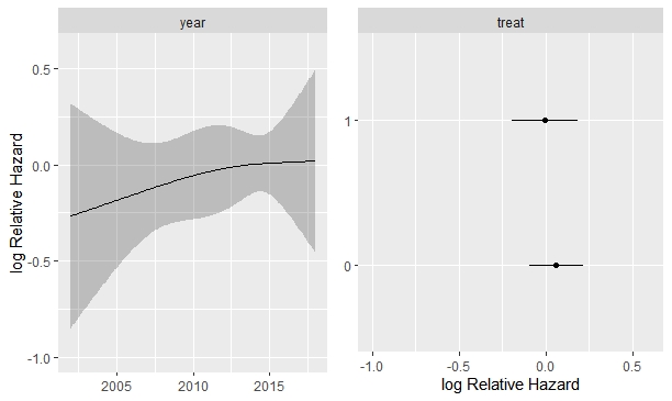
ggplot (Predict(model2), sepdiscrete = “horizontal” , nlevels=2,
vnames = “names” )
In this case, and ignoring that the results are not significant, would the following interpretation be correct?
The increase in years elevates the risk, but only in untreated (treat =0). Is it correct?
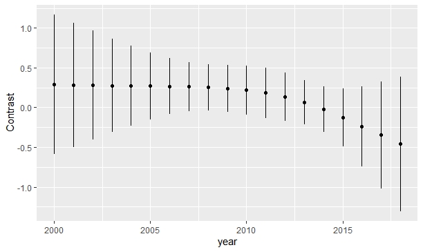
Predict is giving you the treatment effect at the median year, and the year effect for the reference treatment. What you need is Predict(fit, year, treat) to get two curves for the left panel, and a plot of results from contrast() to get the treatment effect as a function of calendar time. Sometimes you need to subject 2000 from year for purely numerical stability reasons. See the help file for contrast.rms for how to use it and how to use lattice or ggplot2 graphics to plot the results with confidence bands.
Let’s see, I leave it here for possible readers of the future. If it’s wrong, correct me, Frank.
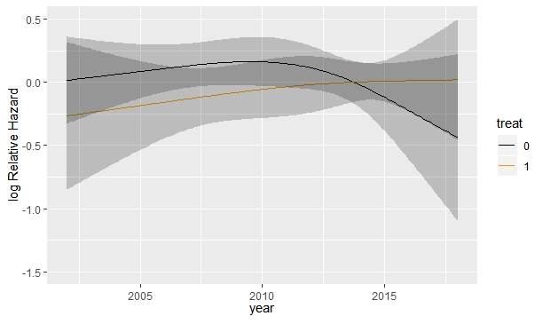
First, the effect of the year, depending on the type of treatment would be as follows: ggplot (Predict(model2,year, treat) )
Would this solution you proposed tease out changes in treatments (e.g., new drugs introduced to the market) or disease management guidelines or policies (access to treatment) over time? Changes in years are potentially discrete events that could wildly impact the outcomes over time (e.g., ACA introduction or new therapy introduced). I understand that splines could remedy some of these issues. My question is how spline perform compared to introducing years as categorical variables? Also, I would assume more censoring would happen in later years partially due to more treatment options (at least in some diseases space like RA)
To the last part of your question, I suggestion thinking about this through the number of knots that you pre-specify. If you think that there can be sudden, large, changes in Y you need more knots, and may want to put two knots near a known calendar time where something “big” happened. Regarding the earlier part of what you wrote, you might model long-term smooth trends with a spline but have indicator variables for specific events suspected to have instant effects.
The contrast function is really powerful, it allows you to explore a large number of issues within the fitted model.
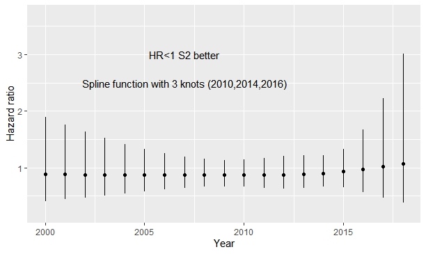
In addition I have put the knots about 2016 as suggested with treat*rcs(year, c(2010,2014, 2016); 2016 was the date in which one of the drugs was approved. After that the possible trend observed in the previous plot disappears. Obviating that the first curve is upside down (in the previous code the reference category was upside down and I added some covariates), the change is remarkable.
My opinion is to keep the time trend, because I think that theoretically it is better to control time although it does not seem to be significant.
Just make sure that you have data to support the region around each knot. Also this is sometimes a case for using AIC to select the number of knots. AIC(fit object) will print AIC. You can run it for 3, 4, 5, 6, 7 default knots.
I have done the AIC of several models with various knots, and the best is with three knots focused on the date of drug approval. I have also seen that the lognormal parametric model fits better than the Cox model, which was to be expected given the situation of non-proportional hazards. However, all these analyses raise me doubts about making decisions about the model specifications with observed effects. For example, some technical documents recommend using AIC or BIC to select the best distribution in parametric models: http://nicedsu.org.uk/technical-support-documents/survival-analysis-tsd/
I have the following question:
Why is this different from selecting covariates according to observed effects?
How is this different from selecting the knots of the splines functions according to AIC?
This is a very interesting issue. If I understood correctly, the goal of this analysis was to estimate the causal effect of a treatment (TxA) on outcome Y. Let’s assume the condition that leads to Y requires constant treatment (i.e. is a chronic condition) and could lead to death. During the period of follow-up there was a change in TxA. The change in TxA has a clinically important effect on Y (otherwise it shouldn’t have been implemented). Let’s call the improved version of TxA as TxB. If the decision to stratify by the time when use of TxB started is substantively justified, wouldn’t you expect the effects of TxA and TxB to be different? Why is it a problem that the two HR were different? Wouldn’t you be more surprised if they were not? On the other hand, if one considers TxA and TxB as a single treatment, then one would be violating the SUTVA assumption (stable-unit-treatment-value assumption), and the effect of TxA would not be identifiable. The magnitude of the average causal effect of the treatment would depend on the proportion of patients who received each version of the treatment (TxA and TxB), the findings will be hard to interpret, and it would be unclear to whom (target population) do they apply. On the other hand, patients who receive TxB are not a random sample of all patients eligible for treatment. To receive TxB patients have to be alive at the time TxB was introduced. Whether they are alive at that time likely depends on whether they were receiving TxA. Thus, inclusion in the study after TxB was introduced is a consequence of both the exposure (TxA) and the outcome (Y–>death). It seems this would introduce selection bias. Thus, even if TxA and TxB had similar effects on the outcome, the estimate of effect in the second time period (after introduction of TxB) would be biased and, therefore, would be different from the effect in the the first period (when only TxA was used). My point is that the answer to this question depends heavily on what TxA and TxB are, what is the outcome, which are the censoring mechanisms, and what assumptions are we making. This goes beyond how to do the statistical analysis.
The two treatments compared here are lanreotide vs octreotide in neuroendocrine tumors. The end point is progression-free survival. I believe that the most plausible reasons for temporary changes in effect may be associated with patterns of use over time, for example, that over time patients receiving one or the other treatment vary, perhaps with residual confounding bias. I found your exposition very interesting and clever. How would it apply to this particular scenario?
I think it does apply. Without pinpointing what those changes are and when they occurred, it won’t be possible to quantify their effect on the relative efficacy of the two treatments. Even if you are certain changes happened in 2012, for example, you still have to deal with the problem of differentiating in which patients the treatment changed (I’m guessing here). If the changes happened for both treatments, then the problem becomes more complicated, because you won’t have a single standard to compare to. Based on the information you provide, I think you could compare the two treatments, using Cox regression analysis, and test for heterogeneity of the effects across calendar time (I’m assuming that’s what you mean when referring to temporary changes). It the efficacy of a treatment, as compared to the other one, changes with calendar time, then you could report what was the effect “before” and “now”, and recommend accordingly (i.e. use as “before” or “now”, depending on which is more beneficial).
Now, I’m assuming changes happened for all patients. However, if it’s the patients themselves that changed over time, for example, if they are diagnosed and treated earlier now than before, then you have two target populations and you may want to carefully consider if the efficacy in both populations would be the same (based on clinical knowledge). Basically, my impression is that all you need to do is a Cox regression analysis (or equivalente) and, if you find heterogeneity of effects across time, try to explain it based on the temporal changes on the way the treatments are used or in the characteristics of the patients that are targeted for treatment now, as compared to before.
I’ve got to get started on this. The constrast function of the rms R package is fabulous, but in my real database there is missing data. Does the contrast function work the same after fit.mult.impute?