Consider a simple example where we investigate the sensitivity of two diagnostic tests by testing the same patients known to be sick using both tests. (For simplicity, I’ll assume everywhere that diagnosis is binary.) Let’s assume that the true value of sensitivity is 0.5 for both tests (i.e., H_0 holds.)
What is the appropriate way to statistically compare the tests? Here are a few options I could think of, allowing potentially correlating values of the two tests:
library(survival)
library(data.table)
library(ggplot2)

simul <- function(n, r) {
  SimData <- data.frame(Subject = rep(paste0("Subject", 1:n), 2),
                        Test = c(rep("Test1", n), rep("Test2", n)),
                        #Result = sample(c("-", "+"), 2*n, replace = TRUE))
                        Result = c(mvtnorm::rmvnorm(
                          n, mean = c(0, 0),
                          sigma = matrix(c(1, r, r, 1), ncol = 2)) > 0))
  SimTab <- table(SimData[SimData$Test == "Test1",]$Result,
                  SimData[SimData$Test == "Test2",]$Result)
  fit <- glm(Result ~ Test, data = SimData,
             family = binomial(link = "logit"))
  c(McNemar = mcnemar.test(SimTab)$p.value,
    McNemarNoContCorr = mcnemar.test(SimTab, correct = FALSE)$p.value,
    ExactMcNemar = exact2x2::exact2x2(SimTab, tsmethod = "central",
                                      paired = TRUE)$p.value,
    CondLogReg = summary(clogit(Result ~ Test + strata(Subject),
                                data = SimData)
    )$coefficients["TestTest2", "Pr(>|z|)"],
    LogReg = summary(fit)$coefficients["TestTest2", "Pr(>|z|)"],
    LogRegClusterBS = lmtest::coeftest(
      fit, sandwich::vcovBS(fit, cluster = ~ Subject)
    )["TestTest2", "Pr(>|z|)"],
    LogRegClusterHC3 = lmtest::coeftest(
      fit, sandwich::vcovCL(fit, cluster = ~ Subject, type = "HC3")
    )["TestTest2", "Pr(>|z|)"])
}

pargrid <- CJ(n = c(24, 50, 100, 200),
              r = c(0, 0.3, 0.5, 0.7, 0.9))

cl <- parallel::makeCluster(parallel::detectCores() - 1)
parallel::clusterExport(cl, c("simul", "pargrid"))
parallel::clusterEvalQ(cl, library(survival))

SimRes <- rbindlist(lapply(1:nrow(pargrid), function(i) {
  data.table(n = pargrid$n[i], r = pargrid$r[i],
             t(parallel::parSapply(cl, 1:1e4, function(j)
               simul(pargrid$n[i], pargrid$r[i]))))
}))

parallel::stopCluster(cl)
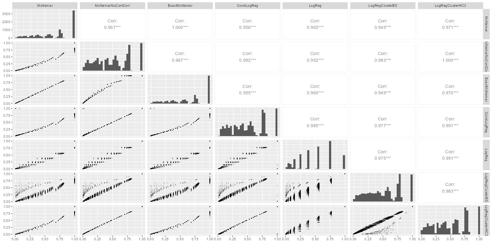
Let’s see the results for uncorrelated tests with a sample size of 24:
GGally::ggpairs(SimRes[r == 0 & n == 24,
                       .(McNemar, McNemarNoContCorr, ExactMcNemar,
                         CondLogReg, LogReg, LogRegClusterBS,
                         LogRegClusterHC3)],
                diag = list(continuous = "barDiag"),
                lower = list(continuous = GGally::wrap(
                  "points", size = 0.1, alpha = 0.3)))
And (again for uncorrelated tests, with a sample size of 24):
cbind(colMeans(SimRes[r==0 & n == 24] < 0.05))
McNemar           0.0255
McNemarNoContCorr 0.0466
ExactMcNemar      0.0262
CondLogReg        0.0302
LogReg            0.0617
LogRegClusterBS   0.0357
LogRegClusterHC3  0.0447
Now, I find this very surprising:
- Simple logistic regression does not account for measurements coming from the same patient, so I assumed it’ll be horribly invalid. Instead it turned out to be acceptable – actually, even better than McNemar’s test which specifically adjusts for this!
- What is probably even more surprising is that adjusting logistic regression for the clustering actually made the situation worse…! (And, as a sidenote, bootstrap seems to be worse than HC3.)
- Just a minor remark compared to these, but I was surprised about the results of conditional logistic regression too – I was under the impression that it is identical to McNemar’s test, but clearly not.
What is the explanation for these? Or I made a mistake in the simulation…?
Update. As pointed out in the comments, the fact that simple logistic regression (which does not correct for correlation) works well is not surprising, as I haven’t assumed that the tests are correlated. (Although it is still strange that it is better than McNemar’s test, or that the correction makes it worse.) Let’s see what de we have for different correlations, with a sample size of 24:
dcast(melt(SimRes[n == 24], id.vars = c("n", "r"))[
  ,.(mean(value < 0.05, na.rm = TRUE)),
  .(n, r, variable)], variable ~ n + r, value.var = "V1")
            variable   24_0 24_0.3     24_0.5      24_0.7     24_0.9
              <fctr>  <num>  <num>      <num>       <num>      <num>
1:           McNemar 0.0255 0.0191 0.01910191 0.013513514 0.00317623
2: McNemarNoContCorr 0.0466 0.0416 0.04450445 0.048048048 0.04098361
3:      ExactMcNemar 0.0262 0.0193 0.01910000 0.013500000 0.00310000
4:        CondLogReg 0.0302 0.0183 0.01060106 0.003403403 0.00000000
5:            LogReg 0.0617 0.0350 0.02350000 0.009000000 0.00030000
6:   LogRegClusterBS 0.0357 0.0350 0.03820000 0.041300000 0.03230000
7:  LogRegClusterHC3 0.0447 0.0413 0.04450000 0.048114434 0.04325085
Now, what I see here:
- Logistic regression indeed gets (much) worse with correlation, so that’s a good news.
- Adjusting it for clustering indeed corrects it (even for the most extreme cases of correlation), at least to that extent what we have seen without correlation. So that’s again good news.
- HC3 now definitely seems to be better than bootstrap.
- The problem is with McNemar: it gets horribly invalid even for moderate correlations. That’s practically impossible as it specifically takes pairing into account, so I suspect an error in the simulation (although I couldn’t find it…).
Update #2. Another point that came up within the comments is that sample size might be relevant, in particular, n=24 is small, which might have an important impact on the result. (Although I thought continuity corrected or exact McNemar’s test should work for small samples too!) Nevertheless, I carried out a more extensive analysis involving different sample sizes:
res <- melt(SimRes, id.vars = c("n", "r"))[
  ,.(mean(value < 0.05, na.rm = TRUE)),
  .(n, r, variable)]
One can get the numerical results with dcast(res, n + variable ~ r, value.var = "V1"), but I now rather plot it:
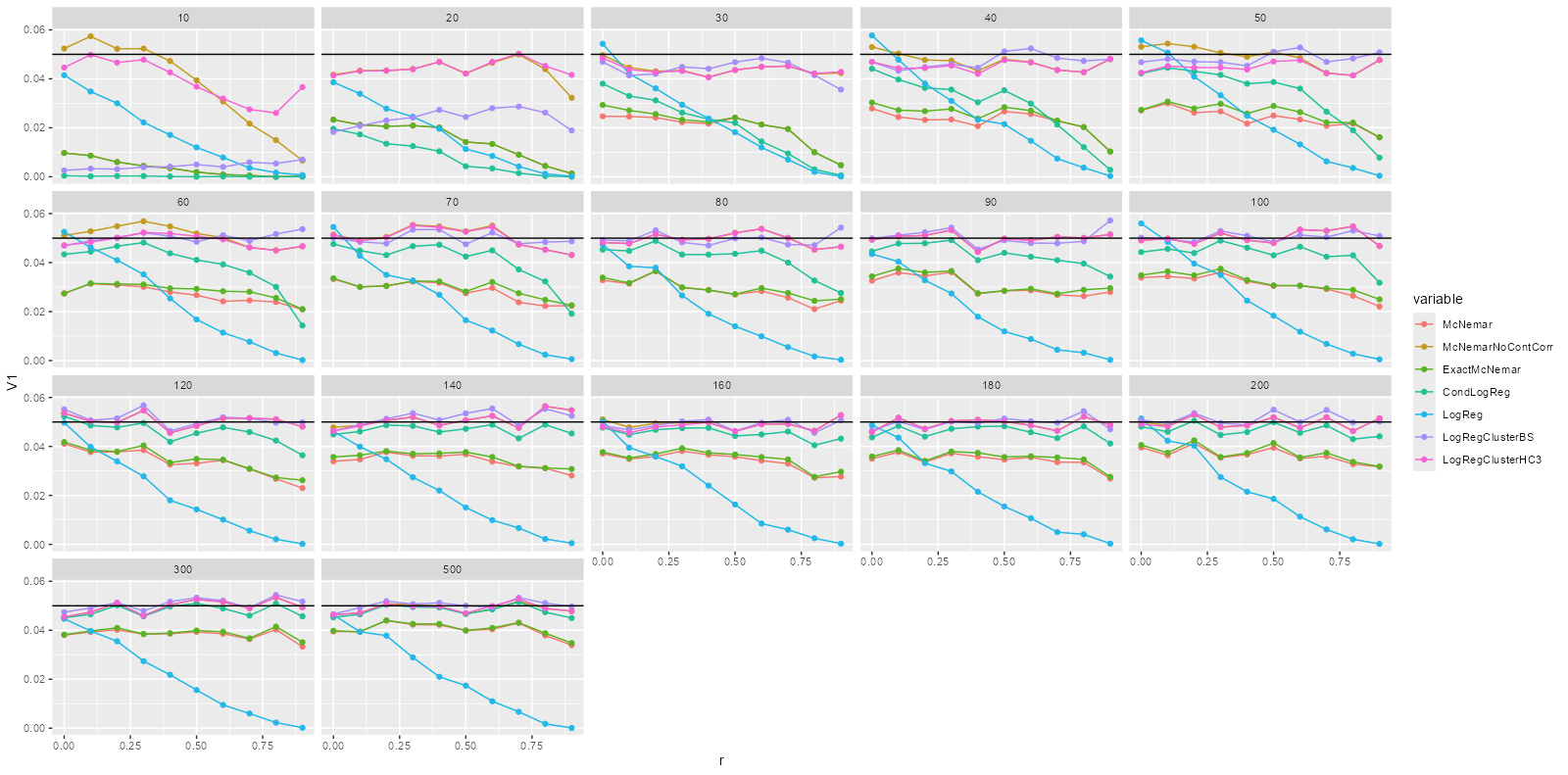
ggplot(res, aes(x = r, y = V1, group = variable, color = variable)) +
  facet_wrap(~n) + geom_line() + geom_point() +
  geom_hline(yintercept = 0.05)
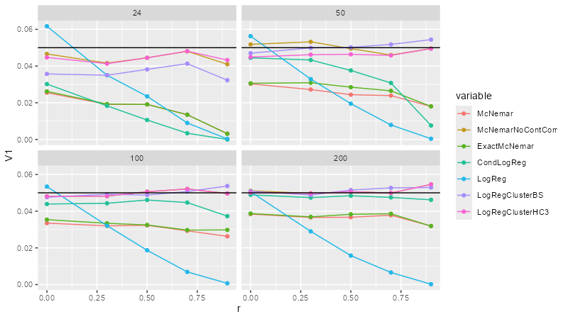
Assuming that there are no bugs in my simulation, a couple of very interesting observations can be made:
- Now everything is clear regarding my initial question: simple logistic regression works well only for no correlation, and gets horrible wrong with correlation.
- What is very surprising (at least to me) that for small samples, the same is true for McNemar’s test, for exact McNemar’s test and for the conditional logistic regression.
- The second thing that I don’t understand at all (to the point that I feel it might be a bug) is that neither McNemar’s test, nor its exact version is good even with a sample size of n=200. Yes, they’re much better than for small samples (in particular, they won’t be really affected by correlation), but far from being OK even with n=200.
- The third thing that is very surprising is that switching continuity correction off makes McNemar’s test much-much better: it works reasonably well for all investigated correlation and samples sizes.
- Perhaps the most surprising is that the overall “winner” is pretty clearly logistic regression with an HC3 adjustment for clustering – this proved to be the best for almost every correlation and sample size (i.e., it surpassed the purpose-built McNemar’s test).
- It might be just a very strange coincide, but I thought I mention that for larger samples sizes logistic regression + HC3 and non-continuity corrected McNemar’s test were almost exactly identical (the binary decisions were the same in every simulation out of 10,000 and the correlation of their p-values was
0.9999976for the sample size of 200). That’s pretty peculiar as – I assumed – they are totally different approaches.