This post based is on concepts described in Chapter 13 of the forthcoming 4th edition of the Oxford Handbook of Clinical Diagnosis. These concepts are based on my attempt to model using probability theory the transparent reasoning processes that I have observed my teachers, my colleagues and myself using during diagnosis and decisions from my time as a student. I discovered that many of these transparent reasoning processes had not been described before or modelled using probability theory. I have included these in the Oxford Handbook of Clinical Diagnosis in order that students, young doctors and statisticians not yet familiar with the diagnostic process can get a head start in improving transparent diagnostic and decision making processes of the future.
The assumption of conditional independence is central to modelling stochastic processes, including games of chance. It is also widely assumed by those in disciplines such as artificial intelligence and machine learning. However, this assumption alone is not enough for some purposes (e.g. during the differential diagnostic process). The hallmark of the differential diagnostic process is that it involves creating a simplifying short list of possible diagnoses conditional on an initiating finding (often described as a ‘lead’) and looking for more individual items of information that make all but one diagnosis in the list improbable. This reasoning can be modelled with a derivation of the extended form of Bayes rule. Single items of information are then sought that occur commonly in one listed diagnosis and less commonly in at least one other diagnosis thus making the former more probable and the latter less probable.
In order to allow for the possibility of one patient having more than one diagnosis, the individual probabilities of diagnoses conditional on the lead are assumed to sum 1 or more (i.e. ≥1). If a combination of findings is present [i.e. *F1∩F2…∩Fn*] and one finding [Fi(min)] occurs rarely or never in those with a diagnostic criterion Dj then the frequency of that combination can be no higher than that single finding that occurs rarely or never [i.e. *p(F1* *∩F2…* *∩Fn|Dj)* *≤ p(Fi|Dj)min*]. If the frequency of the combination is assumed to be EQUAL to that of rarest occurring [i.e. *p(F1* *∩F2…* *∩Fn|Dj) = p(Fi|Dj)min*], then this assumes positive conditional dependence.
If a number n of findings occur in those with a diagnostic criterion Dj or Dx then the minimum frequency of occurrence of the combination is the sum of the individual frequencies minus their number plus one [i.e. *p(F1* *∩F2…* *∩Fn|Dj)* *≥ ∑ᵑ p(Fi|Dx)-n+1].* If a number ‘n’ of findings Fi occur in those with a diagnostic criterion ‘Dj or Dx’ and the frequency of occurrence of the combination is assumed to be EQUAL to the sum of the individual frequencies minus their number plus one [i.e. *p(F1* *∩F2…* *∩Fn|Dj)* *= ∑ᵑ p(Fi|Dx)-n+1],* this assumes negative conditional dependence.
If there are ‘m’ differential diagnoses, when Dx is a postulated diagnosis, when F0 is the initial finding or lead, when D0 is all diagnoses NOT in the list of differential diagnoses from 1 to ‘m’, then without making any assumptions of conditional dependence or independence, we may infer that the probability of a postulated diagnosis must be:
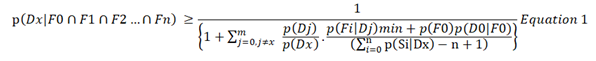
Equation 1 makes no assumptions and is deduced only from the axioms of probability. Note that p(F0).p(D0|F0) replaces p(D0).p(F0|D0) because p(F0).p(D0|F0) = p(D0).p(F0|D0). However, it is possible that the right had side of Equation 1 will be a minus value if ∑ᵑ p(Fi|Dx)-n+1 is a minus value. This may happen because one or more of the values of p(Fi|Dx) is low (e.g. if its is a probability density). The result will unhelpful but still correct as any probability is always greater than a minus value. In order to avoid minus values, we have to make some assumptions.
If we can assume that the contribution of a finding’s likelihood ratio to the probability of a diagnosis in combination with other findings is the same whatever the value of the individual likelihoods (e.g. 0.1/0.2 = 0.5 is equivalent to 0.4/0.8 = 0.5) then this can be termed a ‘likelihood ratio equivalence assumption’. If we also chose the minimum likelihood ratio, then this can be no greater than one if we regard the finding ‘U’ that defines the universal set as a one of the findings to be automatically taken into account so that the likelihood ratio p(U|Dj)/p(U|Dx)min = 1/1 = 1. This means that all likelihood ratios greater than one will not satisfy the condition of being the minimum likelihood ratio available so that if it is greater than one then it will be replaced by one as this will be the minimum available. Therefore, if we make an additional assumption of positive and negative dependence as above and another assumption of likelihood ratio equivalence then:
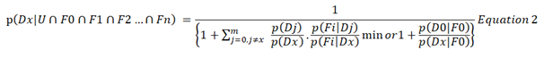
Equation 1 gives a lower bound and thus potentially an underestimate of the probability of a diagnosis. Equation 2 can therefore be expected to do the same. This contrasts with a tendency to over-estimate of probabilities when making an assumption of conditional independence. However, it is still possible to make an assumption of conditional independence for a limited number of findings [e.g. G1 to Gr so that p(Fi|Dj) = ∏ᵑ p(Gh|Dj) and p(Fi|Dx) = ∏ᵑ p(Gh|Dx) for use in Equation 2.
Equation 2 can be rearranged to give:

Equations 2 and 3 simplify calculations from a human point of view because they only expect the user to identify the findings that provide the minimum likelihood ratio for each differential diagnosis. It does not expect the diagnostician to estimate the likelihood ratios of vast combinations of evidence that represents the ‘total evidence’ by assuming conditional independence. This is impossible anyway as it is only possible to estimate the frequencies in those with diagnosis for a limited number of available findings.
The same reasoning can be used to consider a number of scientific hypotheses. However, p(D0|F0)/p(Dx/F0) will not be known when reasoning with scientific hypotheses so that the conclusion will have to be
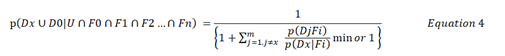
In other words Equation 4 estimates that the probability of the postulate Dx or something else D0 being confirmed in the long run may be at least as high as the right hand side of Equation 4 and the probability of alternative explanations may no higher than one minus the right hand side of Equation 4. In other words, individual scientific hypotheses cannot be confirmed or shown to be probable. It is only their alternatives that can be shown to be improbable (or refuted as asserted by Karl Popper). This can also happen during the diagnostic process when it is not possible to estimate the proportion of patients with a finding that do not have one of the diagnoses in its list of differential diagnoses [i.e p(D0|S0). Equation 4 can therefore be regarded as a model for ‘abductive reasoning’.
The Oxford Handbook of Clinical Diagnosis is based on the reasoning represented by Equations 1 to 4. Chapter 13 provides example data of how they can be applied and there is a formal proof at the end. The examples for the 3rd edition [1] are being improved in the forthcoming 4th edition. I would be grateful for any comments.
References
- Llewelyn H. Proof for the reasoning by probable elimination theorem [in Llewelyn H, Aun Ang H, Lewis K, Al-Abdullah A. The Oxford Handbook of Clinical Diagnosis, 3 rd edition]. https://oxfordmedicine.com/view/10.1093/med/9780199679867.001.0001/med-9780199679867-chapter-13#med-9780199679867-chapter-13-div1-20