I want to share a new method to perform inference on time-series. It allows one to study non-linear patterns in time-series, even in very small data.
The SymbolicInference.jl package applies analytic combinatorics to Recurrence Quantification Analysis objects in order to obtain exact probability distributions for constrained specifications.
The rationale is described in the white paper: Probabilistic inference on arbitrary time-series via symbolic methods: exploring complex dynamics with analytics combinatorics and recurrence analysis.
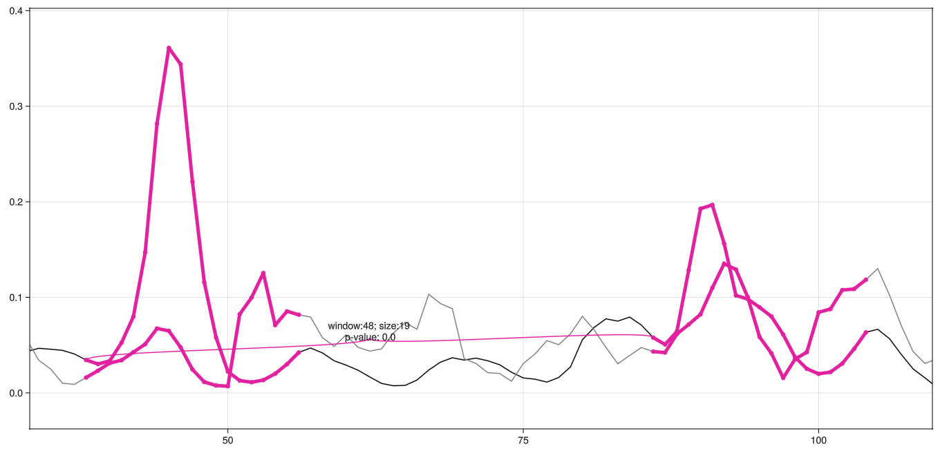
Abstract: Recurrence quantification analysis (RQA) is inspired by Poincare ‘s early studies and describes non-linear characteristics in time-series by identifying similarity between states pairwisely among all observations. Since every pair is either close or distant, this procedure maps trajectories to the realm of binary states, a fruitful field for the application of combinatorial tools. In this work, we leverage symbolic methods from analytic combinatorics to make inference on time-series data. Methods were implemented and made available in open-source software (AnalyticComb.jl ; SymbolicInference.jl). Study cases include simulated data, precipitation volumes and dengue cases. We demonstrate the detection of significant motifs: specific sequences of consecutive states that are repeated within a series or between two of them. The framework successfully identifies patterns in systems such as random walks and noisy periodic signals. When applied to empirical data, it also highlights the association of dengue peaks (e.g. infectious outbreaks) and rainfall seasonality (e.g. weather fluctuation). Using combinatorial constructions tailored for special cases, our method provides exact probabilities for inference in the analysis of time-series recurrences
Without confidence intervals and a way to estimate the needed sample size I’m very cautious in recommending such a method. The type I assertion probability \alpha also needs to be checked by simulation to equal the nominal value.
Thank you for the feedback, @f2harrell !
When you talk about confidence intervals, which parameter are you referring to?
Sample size estimation would definitely be a great thing to have. Not trivial for me though. Do you know of anyone up to this task?
The type I assertion probability α also needs to be checked by simulation to equal the nominal value.
I don’t understand this statement.
You are quoting p-values from the method, so you have to understand how to check \alpha through simulation; otherwise remove all inferential quantities from the output. Re: confidence intervals I was referring to confidence bands for the whole curve.
Re: confidence intervals I was referring to confidence bands for the whole curve.
Which curve? It remains unclear to me.
You are quoting p-values from the method, so you have to understand how to check α through simulation; otherwise remove all inferential quantities from the output.
@f2harrell 
Your phrasing was a bit confusing. I understand it now that what you call ‘nominal values’ are actually the analytically obtained p-values.
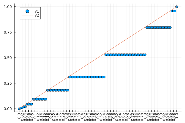
Not at all. Create a situation where the pattern you are trying to detect doesn’t exist and you have a typical amount off randomness. Do this 1000 times, running your algorithm each time. Report the fraction of times the p-value you compute is < 0.05. This fraction estimates the true type I \alpha probability, i.e., it checks whether your p-values are accurate. A fuller assessment is to compute the empirical CDF of the 1000 p-values and show it follows the line of identity; p-values have a U[0,1] distribution under the null hypothesis.
Not at all. Create a situation where the pattern you are trying to detect doesn’t exist and you have a typical amount off randomness. Do this 1000 times…
This confirms what I had in mind.
In that case, the script below does that!
I will add these simulations to the suppl. material.
alpha_thresh, n_series , n_sim = 0.05, 300 , 1000
probs = []
for i in 1:n_sim
cur_array = Random.bitrand(n_series)
arr_enc = StatsBase.rle(cur_array)
max_val = maximum(arr_enc[2])
cur_prob = AnalyticComb.weighted_bin_runs_pval(0.5,0.5,max_val,n_series)
push!(probs,cur_prob)
end
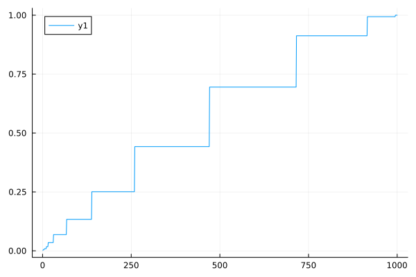
Plots.scatter(sort(probs))
Plots.plot(sort(probs))
pos_vals = map(x -> ifelse(x<alpha_thresh,1,0),probs)
alpha_prop_sim = sum(pos_vals)/length(pos_vals)
When it comes to confidence intervals,
I assume you were mistaken at first (?).
This is not a statistical inference based on an unknown parameter.
You might be thinking about taking sample data to estimate mean (e.g. \overline{\mu} in t-test) or expected proportions and residuals (e.g. \chi^2).
The situation here is closer to Fisher’s “Lady tasting tea”. There’s an exact probability distribution for the sequence of observations at hand. I cannot see where confidence intervals may come in.
Where you thinking of prediction intervals over the time-series because of the visualization?
EDIT: That’s actually a good suggestion. If we think of the number of long-runs as the unknown parameter \overline{l}, it might be possible get a CI for motif size. It would be necessary to have more information about the distribution of long-runs in binary strings related to Equation 5. It also seems feasible to calculate the empirical CIs using the pdfs P(l) plotted in Section IV. A confidence interval on the size of the motifs might actually be informative.
No, I’m just thinking right now that whenever a p-value is provided you need to show that it has the properties of a p-value. The plot you produced is promising, but never using binning in such a calculation. Show the empirical CDF of p-values vs. the p-values, so both axes are 0-1.
There is no binning being done here. The long-runs can only assume integer values (l < n ; l,n \in \mathbf{Z}). The ‘steps’ in the ladder are probabilities associated with common lengths appearing in sequences.
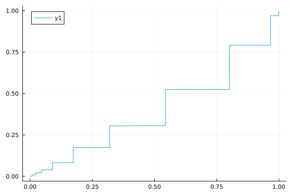
Then it’s not what I was thinking. Show the ECDF of 1000 p-values simulated under the “no signal” situation with x=observed p-value, y=proportion of p-values less than or equal to that observed p-value. Plot the line of identity for reference.
1 Like
This looks odd. P-values computed on continuous data should be continuous. Your p-values have a discrete distribution.
1 Like
Update:
The white-paper outlining this framework was developed and published in an issue of the * The European Physical Journal
It is a nice approach for time-series in which one cannot rely on asymptotic assumptions and want to use exact methods.