Using a proportional odds model instead of logistic model to improve power

I have created a prediction model that outputs a probability that the result of an invasive test alters management, using predictors that are easily obtainable before a decision to perform the invasive test is made. The model is a proportional odds model with four categories; k0, ≥k1, ≥k2, and ≥k3. For historical reasons (although inefficient), only ≥k2 is of any clinical interest and is the only portion of the model that will be used in practice by clinicians. This category is the second smallest category. I chose to use a proportional odds model with all four categories instead of a logistic model with only <k2 and ≥k2 to increase the statistical efficiency of the prediction model given that it is developed on a finite sample. I used the procedure by Richard Riley et al to calculate the minimum required sample size for a logistic model using only <k2 and ≥k2, and demonstrated that the proportional odds assumption held quite well. It is my belief that the model “borrows” information from the practically uninteresting (but much more common) ≥k1 outcome, allowing it to predict the ≥k2 outcome with greater precision.

However, my prediction model has now been returned from revision and I have been asked to simplify the model to a logistic regression or justify the the added complexity associated with using a proportional odds model. I am unable to find any published justification for my belief that the proportional odds model is more efficient and I am having a hard time articulating a rebuttal to the request to simplify to a logistic model. Is my rationale correct and are there any publications I can link to?

I have previously discussed a similar problem, links below.
1 Like

Professor Frank Harrell had previously suggested using popower from the Hmisc package. Despite reading as much as I could and trying to implement myself, I was unable to parse how to do this or interpret the answer. If anyone could build upon this suggestion I would be much obliged.

1 Like

The easiest way out is to compute the standard error of a main parameter of interest (log odds ratio), for 2, 3, or 4 levels. When collapsing 4 original levels into 2 or 3 levels the loss of information is reflected by increased SEs. Show the 3 SEs to the reviewer.

3 Likes

Thank you, I will do this. I have also considered running through the comparison and procedures you outlined in Statistical Thinking - Statistically Efficient Ways to Quantify Added Predictive Value of New Measurements . I know these are not nested models, but would it be entirely ridiculous to compare the models this way, given that both include the same parameters on the same data and are both meant to predict ≥k2? I realise the ordinal model as the added benefit of predicting ≥k1, ≥k2 and ≥3 but there is a strong cultural reason for clinicians not caring about ≥k1 and ≥k3 and this added benefit is of little practical value.

Those methods do apply here, but a little more indirectly. I would instead concentrate on precision and possibly power. Precision is easiest. But likelihood ratio \chi^2 of binary vs. ordinal models is also useful for quantifying information content as you add more levels to Y.

1 Like

This is my attempt at what I believe is a similar rationale.

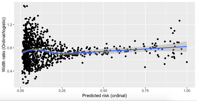
First I calculate the width of the 95% confidence interval of the predicted risk for the k2 outcome from the ordinal model, for all individuals in the dataset.

l_ordinal_risk <- list()
for (i in 1:nrow(df)) {
  ordinal_risk <- Predict(
    fit_ordinal, kint = 2, 
    X1 = as.character(df[i, "X1"]),
    X2 = as.numeric(df[i, "X2"]),
    X3 = as.numeric(df[i, "X3"]),
    X4 = as.numeric(df[i, "X4"]),
    X5 = as.numeric(df[i, "X5"]),
    X6 = as.numeric(df[i, "X6"]),
    fun =plogis)
  ordinal_risk$num <- i
  l_ordinal_risk[[i]] <- ordinal_risk
}

ordinal_risk <- do.call(rbind, l_ordinal_risk)
ordinal_risk$width <- ordinal_risk$upper - ordinal_risk$lower

I then do the same for the binary logistic model, again calculating the width of the interval on the risk scale for each individual.

l_logistic_risk <- list()
for (i in 1:nrow(df)) {
  logistic_risk <- Predict(
    fit_logistic,
    X1 = as.character(df[i, "X1"]),
    X2 = as.numeric(df[i, "X2"]),
    X3 = as.numeric(df[i, "X3"]),
    X4 = as.numeric(df[i, "X4"]),
    X5 = as.numeric(df[i, "X5"]),
    X6 = as.numeric(df[i, "X6"]),
    fun =plogis)
  logistic_risk$num <- i
  l_logistic_risk[[i]] <- logistic_risk
}

logistic_risk <- do.call(rbind, l_logistic_risk)

logistic_risk$width <- logistic_risk$upper - logistic_risk$lower

I then show the distribution of width ratios between the ordinal and logistic models.

quantile(ordinal_risk$width/logistic_risk$width)

And show that the width of the 95% confidence interval of the predicted risk for the ordinal model compared to the logistic model, is a median of 0.73 (IQR 0.60 to 0.86), i.e. 14-40% tighter. I personally find this a very convincing argument for the ordinal approach, unless I am badly mistaken.

2 Likes

This is excellent. The relative efficiency will probably vary with the frequency of outcome levels around the cut point. I do think it’s important to also emphasize the relative efficiency of the two log odds ratio estimates.

Repeating the above on the log-odds scale leads to the whole quantile distribution remaining under 1, with a median width ratio of 0.6, IQR of 0.55-0.67 and 0 percentile of 0.19 and 100 percentile of 0.82. I can’t say I understand how the distribution width ratios differs so between the two scales, but they are at least qualitatively similar.

I am scared that the reviewers will not appreciate the gains in precision and I want to reframe this as, approximately how much larger my sample size would need to be, such that the precision of the logistic regression model would be equivalent to the ordinal model for the current sample size.

Can you think of some way to approximate this?

The ratio of the variances of the two log odds ratios equals the sample size ratio.

1 Like

If I’m understanding you correctly then, if my sample size was 1000 persons for the current precision provided by the ordinal model and the median ‘width ratio’ (which I take to be equal to the ratio of variances) between the confidence intervals of the ordinal and logistic models was 0.6, then the approximate sample size needed for the logistic model to be ‘as precise’ as the ordinal model it would be (1 + (1 - 0.6) )* 1000 = 1400 persons. Am I understanding correctly?

Please excuse my repeated questions, I have tried to read background information about ordinal and logistic models in Regression Modelling Strategies 2nd edition and Categorical Data Analysis by Agresti but I can’t figure out exactly how and why the ratio of variances should equal the sample size ratio

1 Like

That is correct. The general principle is that standard errors are inversely proportional to the square root of the sample size if the Y distribution stays the same.

1 Like

This may merit a separate thread but reviewers of @Elias_Eythorsson’s model may now point out this just published article arguing against the use of the proportional odds model, which is worth discussing. Personally, since I often settle for proportional hazard models for survival outcomes, I am certainly open to proportional odds and also appreciate its higher resolution versus binary outcomes.

Thanks for alerting us to that paper. The paper is very problematic for reasons summarized here. Why didn’t the authors show that estimated hazard ratios vary with time or variances in two treatment groups are unequal? If odds aren’t proportional you can do something about it, but if they are truly not proportional any dichotomization of Y will be arbitrary, besides losing a lot of power.

2 Likes

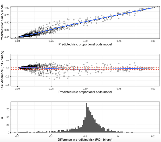
I will read it with interest. However, I have thoroughly examined the proportional odds assumption and I am satisfied that it is more than met and that there are no systematic differences between the predictions made by the ordinal model and the logistic model for ≥k2

2 Likes