What is type I error?

Statisticians, clinical trialists, and drug regulators frequently claim that they want to control the probability of a type I error, and they go on to say that this equates to a probability of a false positive result. This thinking is oversimplified, and I wonder if type I error is an error in the usual sense of the word. For example, a researcher may go through the following thought process.

I want to limit the number of misleading findings over the long run of repeated experiments like mine. I set \alpha=0.05 so that only \frac{1}{20}^\text{th} of the time will the result be “positive” when the truth is really “negative”.

Note the subtlety in the word result. A result may be something like an estimate of a mean difference, or a statistic or p-value for testing for a zero mean difference. \alpha deals with such results. This alludes to the fraction of repeat experiments in which an assertion of a positive effect is made. But what most researchers really want is given by the following:

I want to limit the chance that the treatment doesn’t really work when I assert that it works (has a positive effect).

This alludes to a judgement or decision error — the treatment is truly ineffective when you assert that it is effective.

When I think of error I think of an error in judgment at the point in which the truth is revealed, e.g., one decides to get a painful biopsy and the pathology result is “benign lesion”. So to me a false positive means that an assertion of true positivity was made but that the revealed truth is not positive. The probability of making such an error is the probability that the assertion is false, i.e., the probability that the true condition is negative, e.g., a treatment effect is zero.

Suppose one is interesting in comparing treatment B with treatment A, and the unknown difference between true treatment means is \Delta. Let H_0 be the null hypothesis that \Delta=0. Then the type I error \alpha of a frequentist test of H_0 using a nominal p-value cutoff of 0.05 is

P(test statistic > critical value | \Delta=0) = P(assert \Delta \neq 0 | \Delta=0) = P(p < 0.05)

The conditioning event follows the vertical bar | and can be read e.g. "if \Delta=0". \alpha is 0.05 if the p-values are accurate and the statistical test is a single pre-specified test (e.g., sequential testing was not done).

On the other hand, the false positive probability is

P(\Delta = 0 | assert \Delta \neq 0) = P(\Delta = 0 | p < 0.05)

This false positive probability is arbitrarily different from type I error, and can only be obtained from a Bayesian argument.

My conclusion is that even though many researchers claim to desire a type I error, what they are getting from the type I error probability \alpha is not what they really wanted in the first place. Thus controlling type I error was never the most relevant goal. Type I error is a false assertion probability and not the probability that the treatment doesn’t work.

As as side note, treatments can cause harm and not just fail to benefit patients. So the framing of H_0 does not formally allow for the possibility of harm. A Bayesian posterior probability, on the other hand, would be P(\Delta > 0) = 1 - P(\Delta \leq 0) = P(treatment has no effect or actually harms patients). This seems to be a more relevant probability than P(H_0 is true).

10 Likes

I’d like to suggest that ‘Type 1 error control’ appeals to regulators and researchers as a manufacturing quality control concept. For someone in the business of manufacturing large quantities of regulatory approvals or research ‘findings’, then p < 0.05 means less than 1 in 20 products ‘sold’ will be defective. In a manufacturing setting, a frequentist notion of probability serves just fine.

Of course, as I have noted elsewhere, frequentist probability notions are grossly inadequate for dealing with the problems arising in singular decisions. But in a manufacturing context, where the long-run balance between output and defect rates is chiefly of concern, the frequentist probability concept seems perfectly adapted as an engineering heuristic.

Ford Motor Co’s cost-benefit analysis in the Pinto Memo comes to mind as an example of frequentist, long-run thinking. In the case of regulators (whom you cite), being specific about the utilities and interests involved may be helpful. As ethicist Jessica Flanigan notes [1],

Yet because the FDA is so reliant on legislative and public support, the agency has incentives to craft its approval policies in anticipation of potential public backlash and sanction from elected officials.

My claim would be that here, p < 0.05 helps to limit the incidence of backlash. Rougly speaking, \alpha \approx P(backlash).

As a footnote to your side note, Paul Meehl famously said (speaking of H_0: \Delta = 0) that “the null hypothesis is quasi-always false” [2].

  1. Flanigan J. Pharmaceutical Freedom: Why Patients Have a Right to Self-Medicate. New York, NY, United States of America: Oxford University Press; 2017. [Amazon]

  2. Meehl PE. Theoretical Risks and Tabular Asterisks: Sir Karl, Sir Ronald, and the Slow Progress of Soft Psychology. Journal of Consulting and Clinical Psychiatry. 1978;46:806-834. [PDF]

3 Likes

Thanks, Frank. I had to read twice to follow the logic, but I think I grok.

To make this more concrete for me, are you able to give a real-world example in which the distinction you’re making makes a difference?

Thanks!

2 Likes

David I question even that. \alpha = 0.05 means that if the truth is always zero we expect to make an assertion of a positive effect \frac{1}{20}^\text{th} of the time. It doesn’t mean that one out of twenty will be actually positive.

3 Likes

This occurs so often that I’m disinclined to do that. The number of times decision makers were falsely comforted by a long-term positive assertion probability is staggering, as is the number of times decision makers were falsely alarmed by a large long-term positive assertion fraction. IMHO they like the judge in a court should be concerned with maximizing the probability of making the right decision for the one case in front of them.

3 Likes

I think I’m lost again, sadly. But I will re-read this a few more times & see if I can understand how to apply what you’re saying in a practical instance.

I was taking for granted all many conditions packed into your proviso, “if the p-values are accurate”! Also, by identifying Type 1 error control as an “engineering heuristic,” I intended to emphasize the inexactness of the approach.

1 Like

By the way, if anyone else is able to re-cast Frank’s concept in a concrete example, I would be grateful. For me, sometimes taking the general and making it specific illustrates the general notion more clearly. Not sure what that says about me :slight_smile:

I still think the transposed conditional has sneaked its way into your argument.

1 Like

Great question! I also think that the term “type-I error” is widely misunderstood and abused.

Actually, the type-I error is and acceptance error, not a rejection error. It is the wrong acceptance of the alternative hypothesis (“B”) in a Neyman/Pearson hypothesis (A/B) test. The rate of this type of error is controlled by alpha.

In Fisher’s significance tests, there is no alternative, and the test is not about accepting any hypothesis. It is only to see if there is sufficient data to allow us to reject H0. As there is no real alternative we might wrongly accept, there is nothing like a type-I error in the context of a significance test.

The mess started when significance (rejection-)tests and hypothesis (acceptance-)tests were mixed in “that parody of falsificationism in which straw-man null hypothesis A is rejected and this is taken as evidence in favor of preferred alternative B”, as Andrew Gelman said (The Americal Statistician 2016, Online Discussion on the ASA Statements about p-values).

The significance test is about the data, and H0 is only a mental, theoretical reference point to judge the data. Nothing is won when we say that H0 must be false because the results were “significant” (tiny p-value). This is not the question. The question is rather: is the data we have (already) sufficient to at least show that the model resticted to H0 is obviousely not able to describe the data well? Can we see this (already), clearly enough? At no point is there the question whether or not H0 is true or false.

Similarily for hypothesis tests. There is no statement about the truth and falsehood of the selected hypotheses. And “accepting” one of these alternatives mean, specifically, to “behave as if this alternative was true” (Neyman). It’s not that we would claim this hypothesis being true. It’s only that we should behave as if, and so to minimize the expected loss (or maximize the expected win), as based on the decision strategy.

However, if we see the term “type-I error” as “rejecting H0 under the assumption of H0” (note: I did not use the word ‘wrong’ here!), it makes some (but not much) sense for significance tests. If we never repeat an experiment that failed to be “significant” and we never reject H0 when p > alpha, then we can say that under the assumption of H0 for all our experiments we would not reject H0 (much) more often than alpha*100% of the times. I am not sure if this is a very helpful insight, though. But there is not much more what one can squeeze out of this, without tapping into illogical pitfalls. The best is, to my opinion, to see the p-value as a mere “statistical signal-to-noise ratio”, and to see alpha as a lower limit to identify a “signal” in front of the “noise”. The “signal” is relative to the chosen H0, and the “noise” depends on the variance of the data as well as on the sample size.

my 2p

.

8 Likes

Thank you for this explanation. This is helpful.

I added an example at the beginning which I hope helps.

2 Likes

Thank you. Regarding your biopsy example, is the idea that it is an error to biopsy something that is benign (which, of course, one must do sometimes to find that which is not benign)? That could be an error in one frame of thought, and could be perfectly reasonable at the same time? As the old saying goes: “if you’re not removing any normal appendices, you’re missing some appendicitis.”

Not sure my appendicitis example is a terrific one because maybe it’s OK to miss appendicitis sometimes


1 Like

errors

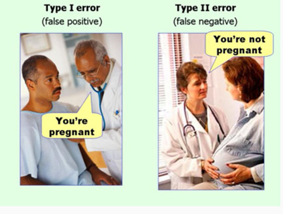
The way I see it, the attached picture is wrong because the type I error would be: P(A | B) in a long-run repeat that assumes B

Whereas false positive would be: P(B | A)

Whereby:
A: saying “you are pregnant”
B: the person is not pregnant

For individual decision making we are usually more interested in the false positive (which in a way is the inverse probability of what the type I error is).

3 Likes

How do you approach pre-study power estimation in a frequenist’s paradigm if you find α constructs of limited value?

1 Like

Frank, by insisting on singular probabilities here, you risk making a circular argument. Of course as you know I have zero sympathy with frequentist probability notions in medicine. Ultimately, they spawn unethical ideas and morally wrong actions. For example, everyone ought to abhor the long-run frequentist thinking that 1-size-fits-all dose-finding methodologists (the so-called OneSizeFitsAllogists) indulge in when they aim to achieve a given ‘target toxicity rate’ in dose-finding trials.

1 Like

You raise a great question. The whole idea of error is something we can question. An analogy: a US Weather Service rainfall forecast of probability of rain of 0.3 when it doesn’t rain - is that an error? The way the USWS scores it is using the Brier score so it’s an amount of error of 0.3^2. We need better terminology that is more judgment-free. Nominations welcomed! I’d like to focus on terminology such as “the chance that y happens if we observe x is z”.

5 Likes

I like your suggested phrase and the overall point you’re making!

1 Like

I’m thinking it was more like the Ergodic Hypothesis :wink:

Nice question. Pre-study power is useful if you don’t have time to be Bayesian. By pretending the effect \Delta to detect is known and is a constant, and making other simplifying assumptions, we can compute n such that Prob(p < 0.05 | \Delta) is 0.9 or so. Better than not computing it and guessing n out of thin air. But more relevant, easier to conceptualize, and honest is to compute Bayesian power: P(posterior probability > 0.9 | entire prior distribution for \Delta). Even more important, Bayesian studies can proceed with no sample size calculation, and proceed until a posterior probability target is reached.

4 Likes