Regression Modeling Strategies: Describing, Resampling, Validating, and Simplifying the Model
This is the fifth of several connected topics organized around chapters in Regression Modeling Strategies. The purposes of these topics are to introduce key concepts in the chapter and to provide a place for questions, answers, and discussion around the chapter’s topics.
This is a key chapter for really understanding RMS.
Section 5.1.1, pp.103
“Regression models are excellent tools for estimating and inferring associations between X and Y given that the “right” variables are in the model.” [emph. dgl]
[Credibility depends on]…design, completeness of the set of variables that are thought to measure confounding and are used for adjustment, … lack of important measurement error, and … the goodness of fit of the model.”
…“These problems [interpreting results of any complexity] can be solved by relying on predicted values and differences between predicted values.”
Other important concepts for the chapter:
Effects are manifest in differences in predicted values
The change in Y when Xj is changed by an amount that is subject matter relevant is the sensible way to consider and represent effects
5.1.2.1 Error measures and prediction accuracy scores include (i) Central tendency of prediction errors, (ii) Discrimination measures, (iii) Calibration measures.
Calibration-in-the-large compares the average Y-hat with the average Y (the right result on average). Calibration-in-the-small (high-resolution calibration) assesses the absolute forecast accuracy of the predictions at individual levels of Y-hat. And calibration-in-the-tiny (patient specific).
Predictive discrimination is the ability to rank order subjects; but calibration should be a prior consideration.
“Want to reward a model for giving more extreme predictions, if the predictions are correct”
Brier Score good for comparing two models but absolute value of Brier score is hard to interpret. C-index OK for evaluating one model, but not for comparing models (C-index not sensitive enough).
“Run simulation study with no real associations and show that associations are easy to find.” The Bootstrapping Ranks of Predictors (rms.pdf notes section 5.4 and figure 5.3 is an elegant demonstration of “uncertainty”. This improves intuition and reveals our biases toward “over-certainty.”
Brier Scaled as an alternative to Brier Score for an easier interpretation? Extract from the Steyerberg (2010) manuscript (DOI: 10.1097/EDE.0b013e3181c30fb2).
The Brier score is a quadratic scoring rule, where the squared differences between actual binary outcomes Y and predictions p are calculated: (Y-p)^2. We can also write this in a way similar to the logarithmic score: Y x (1- p)^2 + (1-Y) x p^2. The Brier score for a model can range from 0 for a perfect model to 0.25 for a noninformative model with a 50% incidence of the outcome. When the outcome incidence is lower, the maximum score for a noninformative model is lower, eg, for 10%: 0.1 x (1 - 0.1)^2 + (1 - 0.1) x 0.1^2=0.090. Similar to Nagelkerke’s approach to the LR statistic, we could scale Brier by its maximum score under a noninformative model: Brier scaled = 1 – Brier/Brier max, where Brier max = mean (p) x (1 - mean (p)), to let it range between 0% and 100%. This scaled Brier score happens to be very similar to Pearson’s R2 statistic
Do you have a good source for interpreting R2 type measures in nonlinear context? Say for dose-response? Papers by Maddala et al in econometrics.
Can we use the validate() function in rms to get optimism corrected c-index? Yes; back-compute from Dxy.
I wonder why RMSE hasn’t been mentioned as a measure for model fit –which is often used in ML. It’s fine, for continuous Y, and is related to R^2.
Should we add model-based description to the other 3 regression strategies? Yes
Does anyone have a reference for Steyerberg’s paper studying p > 0.5 not being quite so damaging for variable elimination from a model? I think the RMS book has the reference.
For the losers vs winners example, seems like you are comparing a model with 10 df for the winners with a model with 990 df with the losers. Would R^2 be a fair comparison between these two models? Yes if the 990 model is penalized or the R^2 is overfitting-corrected.
Do you know of any literature that highlights the issues with the Charlson Comorbidity index? We use it a lot and I’d like to have a reference to bring to my supervisor if possible! (Unsure where this question should be placed, but we brought it up in the validation section ). See the Harrell Steyerberg letter to the editor in J Clin Epi.
Would you recommend bootstrapping ranks of predictors in practice instead of FDR corrected univariate screening?
We mentioned today that c-index performs well in settings with class imbalance, but I found a paper that tries to argue that AUROC is suboptimal in the case of class imbalance (The Precision-Recall Plot Is More Informative than the ROC Plot When Evaluating Binary Classifiers on Imbalanced Datasets, Saito & Rehmsmeier 2015). Am I missing something basic here where c-index is different from AUC?
If I were using repeated Cross Validation to estimate a performance metric (e.g. PPV) that would be used to determine a cutoff of the model score for selecting patients more likely to benefit from treatment in a future trial, what should I use as my confidence intervals for the performance metric? To clarify, I envision a figure with model score (trained from model using continuous versions of biomarkers of course) on the x-axis and performance on the y-axis. I see 2 options:
Empirical distribution of performance metric estimated from each of the repeats of the Cross Validation (this confidence interval would reflect uncertainty in the validation, but not necessarily in the actual performance metric calculated in any given prediction)
Use some version of binomial approximation to estimate confidence interval of performance metric for the median cross validation result.
Which confidence interval do you think is preferred (if any)?
Thanks.
There are several big issues here. First, the benefit on an absolute risk or life expectancy scale, for almost any treatment, will expand as the base risk increases. This is a smooth mathematical phenomenon and doesn’t necessary require any data to deduce. So depending on what you mean by benefit just choose higher risk patients. Second, there is no threshold no matter how you try to define it. Treatment benefit will be a smooth function of patient characteristics with no sudden discontinuity. Performance metrics don’t relate to any of this. Differential treatment benefit is somewhat distinct from resampling validation.
Let me clarify. I am comparing 2 treatments (drug vs placebo). There is an interaction with treatment in the model and a binary outcome. I am using PPV to assess the proportion of actual responders at a given threshold. We are trying to find a reasonable cutoff to select patients with baseline score at an acceptable prevalence level. The x-axis will actually be the difference in score between the two treatment groups, the y-axis will be performance.
No, this will not work. There is no way to tell who responded unless you have a multi-period crossover study and so you observe each patient multiple times under each treatment. PPV only applies to trivial cases where there is a single binary predictor. Cutoffs play no role in anything here, and performance doesn’t either.
Ok. Considering we observe an interaction with treatment in our model. How would you recommend using that information to select patients in future trials who would be more likely to respond to treatment?
Greetings all. I have a process question. I (clinician researcher) am working with statisticians to create a risk prediction model for a binary outcome in a large registry with missing data. We used MICE to impute the missing data, then the ‘fit.mult.impute’ function in ‘rms’ to run the logistic regression using the imputed datasets. We then did internal validation using bootstrapping of this process. Given a little overfitting, we are interested in doing uniform shrinkage of our regression parameters using the bootstrapped calibration slope value. Question is, we cannot find methods to reasonably perform the shrinkage across the imputed datasets. I welcome any and all thoughts on this approach. Thanks in advance.
I have a general question regarding calibration plots that I can’t find a description of in Regression modelling Strategies, 2nd edition, Clinical Prediction models A Practical Approach to Development, Validation, and Updating, Cross Validated nor in other relevant papers. How should one interpret apparent miscalibration at the extremes of predicted values that are not practically relevant for the intended use of the prediction model?
Let’s say a prediction model has been developed that is based on logistic regression. We supply clinicians with continuous predicted probabilities and perform a decision curve analysis knowing the approximate cut-offs of probability that clinicians will be using to guide their decisions. For argument’s sake, let’s assume that most clinicians will consider giving a treatment if a patient’s predicted probability of experiencing the outcome is larger than 10-20%. The calibration plot for this particular model is optimally calibrated between predicted risks of 0% to 40%, but at and above 50% predicted risk the relationship between predicted risk and the LOWESS smooth of actual risk is almost horizontal. Should we consider this model miscalibrated in light of its intended use?
There is a logical flaw in that setup: you require unanimity of clinicians’ thresholds and you won’t find it.
But to your question you can ignore extreme tails where there are almost no data, with the exception that you’d need to mention that if future predictions ever appear in such tails such predictions are of unknown accuracy.
I am trying to get calibration curves for my time-to-event model in an external, “geographically distinct” validation cohort, but I find it difficult to test whether I have done the analysis the right way. Although changing the newdata to the derivation set and also define the survival object from this set gives a near straight diagonal line, it appears the probabilities are not 100% concordant (small deviation), and there is a “overestimation dip” at high pred/obs probabilities. Thus not really sure if the code is working as intended.
Below I try to evaluate calibration at 6 years in the external data. Is the code correct?
fit <- cph(Surv(time,event)~x1+x2, deriv_df, x=TRUE, y=TRUE) # pre-specified model fitted on the derivation data

estim_surv <- survest(fit,
                       newdata=test_df, # geographically distinct cohort but same care setting
                       times=6)$surv # years

ext_val <- val.surv(fit,
             newdata=test_df,
             u=6,
             est.surv=estim_surv,
             S= Surv(test_df$time , test_df$event))

plot(ext_val, xlab="Predicted probability at 6 years", ylab="Observed probability at 6 years", las=1)
Also, does one have to specify u, and e.g. show calibration plots for multiple time points, or is there a way to illustrate calibration across all time points using rms? Both cohorts have ~300 patients of which ~150 have a recorded event within the FU. Many thanks in advance.
You appear to be doing this correctly. I take it that your concern comes from an imperfect calibration plot when evaluated on the training sample. This can definitely happen. The overall slope on the log-log S(t) scale will have to be 1.0 in that case but you can see deviations somewhere along the whole curve.
You can’t automatically get validations at multiple time horizons. You’ll have to run those in a loop and save the results and customize a multi-curve plot. Adding add=TRUE, riskdist=FALSE to all but the first call to plot() will help.
Many thanks! Indeed that was my concern, but good to know it does not have to be 100% calibrated when fitting on the same data used to train.
Does the plot() of a val.survh object fit a loess line on the stored values in p vs. actual and add a histogram of p (the riskdist 1-dimensional scatter plot)? I am wondering because I would like to extract the probability values and plot using ggplot since it is more flexible than base.
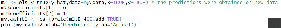
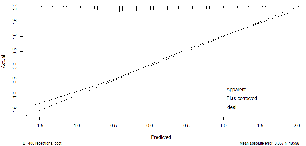
Is it OK to use calibrate() to assess how well a model that was not fitted with rms (support-vector machine) is calibrated over the range of predictions?
For the goodness-of-fit evaluation, I set the coefficients of the intercept and y_hat to 0 and 1, respectively, but I am not sure that this is a correct solution. I have tried to define an explicit formula for this purpose, but could not figure how to do it.
I am currently working on internally validating new prognostic models for event free survival using optimism corrected bootstrapping using 500 bootstrap samples. To do this, I had used the validate function from the rms package in r on a univariate Cox Proportional Hazards model using the prognostic index (risk score). I receive the following output for one of my models at 5-years:
index.orig
training
test
optimism
index.corrected
n
Dxy
0.6986
0.6971
0.6986
-0.0015
0.7001
R2
0.2549
0.2546
0.2549
-0.0003
0.2552
Slope
1.0000
1.0000
1.0039
-0.0039
1.0039
D
0.1112
0.1108
0.1112
-0.0004
0.1116
U
-0.0003
-0.0003
0.0002
-0.0005
0.0002
Q
0.1116
0.1112
0.1111
0.0001
0.1115
g
1.4889
1.4872
1.4889
-0.0017
1.4906
From the output, the optimism corrected calibration slope is 1.0039, which is different from the mean coefficient from the univariate model of 0.0422. The rms package documentation mentions the following regarding calibration slopes ‘The “corrected” slope can be thought of as shrinkage factor that takes into account
overfitting.’ Could you please advise on how the calibration slope was calculated using the validate function in r?
Welcome to datamethods Anita. I don’t think we’ve had this topic come up before. The way that overfitting happens is that when we look at extremes of predictions (X\hat{\beta}) we find that very high predictions are too high after we’ve sorted predictions from low to high ( and low predictions are too low). The sorting from low to high is very reliable when you have a single predictor, and not so reliable when you have lots of predictors so that you have to estimate a lot of regression coefficients that go into the sorting. When you have one predictor, the sorting has to be perfect except in the rare case of getting the wrong sign on the regression coefficient. Any index such as D_{xy} that depends only on the rank order of X\hat{\beta} will show no overfitting. Only absolute indexes such as slope and intercept can show any telltale sign of overfitting, and even then this will be very slight.
All of that is assuming X is fitted with a single coefficient, which means you are assuming it has a linear effect. If you don’t want ot assume that, and you fit a polynomial, spline, or fractional polynomial to X you’ll find a bit of overfitting if your number of events is not very large.
My take-home message is that with a single candidate predictor (i.e., you did not entertain any other predictors) it’s best to relax the linearly assumption unless you know from the literature that the effect is linear on the linear predictor scale, fit that model, and check the proportional hazards (or whatever assumption depending on which survival model you are using) assumption, but not do a formal validation.
I’m doing clinical predictive studies with help of logistic
regression and Cox regression using Harrell’s rms and Hmisc packages.
More precisely, I use lrm and cph but also glm(binomial) and coxph from R and survival.
I have some, probably elementary, questions to help me to proceed. I
use aregImpute for imputation and carry on with fit.mult.impute
to get the averaged model and further use validate and plot(calibrate) to estimate the “optimism in the performance
measures” and the “calibration” of the averaged model. So, what is
actually bootstrapped (with validate and plot(calibrate)) in this
situation: the original data with missing values?, each and every
imputed dataset?, or something else? I assume that the “optimism in
performance measures” and the “calibration” of the averaged model are
reflected in the result from validate and plot(calibrate) as an
internal validation of the results from the original data with missing
values???
Is there an “easy and meaningful” way to add confidence intervals (or
bands) to the plot(calibrate) graph för lrm?
How can predicted (or fitted) individual survival be calculated
(including the basic survival and the effects of the coefficients for
the individual subject) in cox regression in this situation
(imputation and averaging imputed data to results for the model)?
For cph?
For coxph? I realize that I must correct the standard errors with
the covariance-matrix from the fit.mult.impute for coxph and glm(binomial), but except for that, how do I get fitted (predicted)
individual survival? After the correction of the standard errors. I
have no longer a model to use for the “predict” function?
With thanks in advance for any help
Fredrik Lundgren
PS. I hope I have coped correctly to the suggestion from f2harrell. DS
 ). See the Harrell Steyerberg letter to the editor in J Clin Epi.
 Would you recommend bootstrapping ranks of predictors in practice instead of FDR corrected univariate screening?