GD Perkins et al presented an extremely well designed and conducted double blind randomized trial of epinephrine vs. placebo, randomizing over 8,000 patients. The primary outcome was the probability of survival at 30 days. Secondary outcomes included the probability of survival until hospital discharge with a score of 3 or less on the modified Rankin scale (which ranges from 0 [no symptoms] to 6 [death]). The statistical analysis was state-of-the-art, including an ordinal analysis with the proportional odds ordinal logistic model, and Bayesian analysis. The conclusion was that epinephrine increased the chance of survival but among survivors, there was a tendency for worse neurological outcomes. Reaction on twitter (see also here) has been interesting, with some clinicians emphasizing the Rankin score outcomes on survivors. It’s always tricky to interpret conditional analyses, and as one tweet said, there is a relationship between brain damage and risk of death.
A shortcoming of the original analysis in my view is that (1) it’s unclear exactly how the proportional odds analysis was done, and (2) it is not clear that the authors ever performed the preferred ordinal analysis that did not group any outcome levels. A key analysis in the paper combined the bottom 4 levels of the Rankin scale.
Failure to distinguish these categories is not a great idea. Grouping loses information and power. An excellent re-analysis by Matthew Shun-Shin considered full 7-level ordinal analyses with various re-arrangements of the Rankin categories to assume that some neurocognitive outcomes are worse than death. A gold-standard analysis would elicit utilities for all the outcome states from relevant persons and test whether epinephrine increases the expected utility. Short of that, ordinal analyses are better than binary analyses as demonstrated here and here. ![]()
Here is an analysis that uses all 7 categories in their original order, using R.
a <- c(rep(0,15), rep(1,10), rep(2,29), rep(3,20), rep(4,8), rep(5,8), rep(6,3904))
b <- c(rep(0,12), rep(1,17), rep(2,23), rep(3,35), rep(4,12), rep(5,27), rep(6,3881))
x <- c(rep('placebo', length(a)), rep('epinephrine', length(b)))
y <- c(a, b)

require(rms)
f <- lrm(y ~ x)
f

Logistic Regression Model

 lrm(formula = y ~ x)

 Frequencies of Responses

    0    1    2    3    4    5    6
   27   27   52   55   20   35 7785

                      Model Likelihood     Discrimination    Rank Discrim.
                         Ratio Test           Indexes           Indexes
 Obs          8001    LR chi2      5.88    R2       0.003    C       0.541
 max |deriv| 6e-12    d.f.            1    g        0.168    Dxy     0.082
                      Pr(> chi2) 0.0153    gr       1.183    gamma   0.165
                                           gp       0.002    tau-a   0.004
                                           Brier    0.013

           Coef   S.E.   Wald Z Pr(>|Z|)
 y>=1      5.5342 0.2014 27.47  <0.0001
 y>=2      4.8376 0.1485 32.57  <0.0001
 y>=3      4.1565 0.1139 36.48  <0.0001
 y>=4      3.7315 0.0988 37.77  <0.0001
 y>=5      3.6118 0.0953 37.90  <0.0001
 y>=6      3.4304 0.0905 37.90  <0.0001
 x=placebo 0.3368 0.1398  2.41  0.0160

summary(f, x='placebo')

             Effects              Response : y

 Factor                  Low High Diff. Effect   S.E.    Lower 0.95 Upper 0.95
 x - epinephrine:placebo 2   1    NA    -0.33675 0.13985 -0.61085   -0.06266
  Odds Ratio             2   1    NA     0.71408      NA  0.54289    0.93926
The 2-sided (why?) p-value is 0.015 in favor of epi, and the odds epi:placebo OR is 0.71. This provides evidence that patients getting epi tended to have better outcomes on the 7-point scale than those randomized to placebo.
Along the lines of Shun-Shin, let’s assume that modified Rankin scale level 5 is worse than death, and get a new 7-level ordinal analysis:
y2 <- ifelse(y == 5, 7, y)
f <- lrm(y2 ~ x)
f

Logistic Regression Model

 lrm(formula = y2 ~ x)

  Frequencies of Responses

    0    1    2    3    4    6    7
   27   27   52   55   20 7785   35

                      Model Likelihood     Discrimination    Rank Discrim.
                         Ratio Test           Indexes           Indexes
 Obs          8001    LR chi2      0.02    R2       0.000    C       0.502
 max |deriv| 2e-07    d.f.            1    g        0.010    Dxy     0.005
                      Pr(> chi2) 0.8843    gr       1.010    gamma   0.010
                                           gp       0.000    tau-a   0.000
                                           Brier    0.013

           Coef    S.E.   Wald Z Pr(>|Z|)
 y>=1       5.6982 0.2049  27.81 <0.0001
 y>=2       5.0016 0.1532  32.64 <0.0001
 y>=3       4.3206 0.1200  36.01 <0.0001
 y>=4       3.8957 0.1057  36.85 <0.0001
 y>=6       3.7760 0.1025  36.86 <0.0001
 y>=7      -5.4176 0.1827 -29.66 <0.0001
 x=placebo -0.0201 0.1379  -0.15 0.8843

summary(f, x='placebo')

             Effects              Response : y2

 Factor                  Low High Diff. Effect  S.E.    Lower 0.95 Upper 0.95
 x - epinephrine:placebo 2   1    NA    0.02007 0.13795 -0.25030   0.29044
  Odds Ratio             2   1    NA    1.02030      NA  0.77857   1.33700
Now we don’t have evidence for benefit of epi (p=0.88) but we also do not have evidence for non-benefit of epi, since the confidence interval on the odds ratio is wide.
Interpretations of clinical trials with nontrivial outcomes are always nuanced!
Note that the above analyses were unadjusted for baseline covariates, due to non-availability of the raw data. Adjusted analyses are more appropriate.
Conclusions
With an ordinal outcome, frequentist statistical power and limiting effective sample size are largely determined by the total of the frequencies of the non-dominant outcome categories. Unless Rankin level 5 is counted as more favorable to patients than death, and absent a full patient utility analysis, the study’s sample size was insufficient for drawing firm conclusions. There were not enough survivors.
What Would a Bayesian Design Do Differently? ![]()
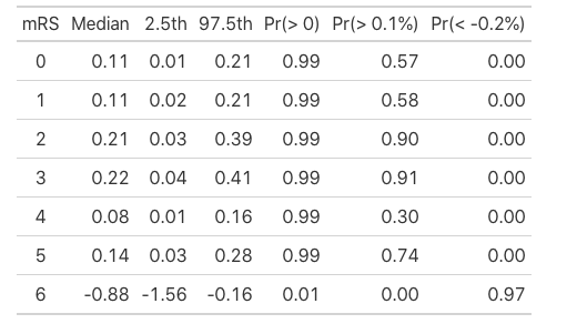
Frequentist designs invite fixed sample sizes, and sample size computation requires knowledge that is not available during study planning. With a Bayesian approach, sampling can continue until a target (efficacy, harm, or futility) is reached, with no penalty for multiple looks. Studies that ended equivocally in the frequentist paradigm can readily be extended in the Bayesian paradigm, subject to resource limitations. Bayesian analysis can also provide some advantages. For example, one can compute the posterior probability that epinephrine reduces mortality by some small, but nonzero, amount.
Other Analyses
G Howard et al provide an exact randomization Wilcoxon test for analyzing all levels of the Rankin score. This is more computationally involved than the proportional odds model and does not allow for covariate adjustment.
Anupam Singh provides an assessment of the proportional odds assumption for this study. The proportional odds assumption is always violated, so one needs to ask whether the weighted average odds ratio arising from the PO model is worse than other overall treatment summaries that may be computed. To quote Stephen Senn:
Clearly, the dependence of the proportional odds model on the assumption of proportionality can be overstressed. Suppose that two different statisticians would cut the same three-point scale at different cut points. It is hard to see how anybody who could accept either dichotomy could object to the compromise answer produced by the proportional odds model.