Most statisticians I’ve spoken with who frequently collaborate with investigators in doing frequentist power calculations believe that the process is nothing more than a game or is voodoo. Minimal clinically important effect sizes are typically re-thought until budget constraints are met, and investigators frequently resort to achieving a power of only 0.8, i.e., are happy to let type I error be 4\times the type I error probability. As a study progresses, the problem re-emerges when doing conditional power calculations that use a mixture of data observed so far and the original effect size to detect.
Statisticians brought up in the frequentist school are often critical of Bayesians’ needing to choose a prior distribution, but they seldom reflect upon exactly what a power calculation is assuming. The use of a single effect size, as opposed to using for example the 0.9 quantile of sample size over some range of effect sizes, has a large effect on the design and interpretation of clinical trials. Bayesian analyses do not use unobservables in their calculations. Sure there is a prior distribution, but this represents a range of plausible values, and doesn’t place emphasis on a single value if the prior is continuous (which I recommend it should be).
Bayesian power is a simpler concept than frequentist power. Given a prior distribution and a design and a schedule for data looks (in a sequential study), Bayesian power can be defined in at least 4 ways, with the first one below being the simplest. (Thanks to Andy Grieve for providing the last two in his reply below).
- the probability that the posterior probability of efficacy will reach or exceed some high level such as 0.95 over the course of the study (if sequentially analyzed) or at the planned study end (if only a single unblinded data look is to be taken)
- the probability that a credible interval exclude a certain special value such as zero efficacy (as in the example below)
- use the predictive distribution of the data
- use the average of the power conditional on a given parameter value with respect to the prior distribution of the parameter
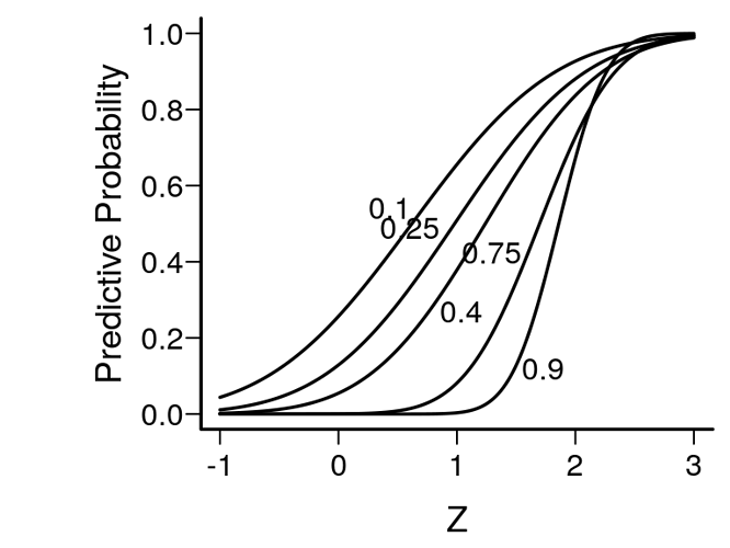
Spiegelhalter, Freedman, and Parmar provide a very elegant example of Bayesian thinking and how it avoids unobservables in a setting in which conditional frequentist power might have been entertained to decide whether a study should be stopped early for futility. Spiegelhalter et al have a very insightful equation that for a simple statistical setup and a flat prior estimates the chance of ultimate success given only the Z-statistic at an interim look that was based on a fraction f of subjects randomized to date. This is shown in the figure below, following by the R code producing the figure. Spiegelhalter et al take issue with the practice of stochastic curtailment or conditional power analysis that assumes a single value of the true unknown efficacy parameter. This Bayesian predictive approach requires no such choice.
Predictive probability of the final 0.95 credible interval excluding zero, and the treatment effect being in the right direction, given the fraction f of study completed and the current test statistic Z when the prior is flat. f values are written beside curves.
require(Hmisc)
pf <- function(z, f) pnorm(z/sqrt(1 - f) - 1.96 * sqrt(f) / sqrt(1 - f))
zs <- seq(-1, 3, length=200)
fs <- c(.1, .25, .4, .75, .9)
d <- expand.grid(Z=zs, f=fs)
f <- d$f
d$p <- with(d, pf(Z, f))
d$f <- NULL
p <- split(d, f)
labcurve(p, pl=TRUE, ylab='Predictive Probability')
