Calibration of Cox model

Madhu · October 22, 2018, 4:16am

I am using Cox model for risk prediction, and I am kind of lost regarding calibration. I am reading on Nam D’Agostino test, but I am unable to grasp the time period to be selected for calculating predicted probabilities. The predicted probabilities vary depending on the time period I select for calculating the probabilities, which directly affects my observed vs predicted probabilities/rates across deciles. I was thinking of using the mean follow-up time in the data to calculate predicted probabilities but a post on statsexchange recommended against using it. I am not sure how to go about this.

(I am using administrative claims data with significant right censoring. Because the enrollment information is month-to-month, my predicted probabilities are monthly)

Thank you.

f2harrell · October 22, 2018, 11:53am

It is not appropriate to use deciles or any other binning of continuous predicted values. My RMS book and course notes go into details related to obtaining smooth semi-parametric calibration curves for survival models, for a single time horizon. This is implemented in the R rms package calibrate.cph function. For examining the entire range of times and not selecting a single time point, there are residual-based methods you may want to take a look at, e.g., see the R rms package val.surv function.

lif · November 17, 2020, 8:28am

Dear Professor,

I developed an AFT log-normal model with the help of your great tutorial RMS book, however I get stuck when I am trying to externally validate the model using a dataset from another country, I think I should use the val.surv function for calibration, but I cannot find any examples illustrating external validation using val.surv, could you please give me a hand? Many many thanks!
feng

f2harrell · November 17, 2020, 11:56am

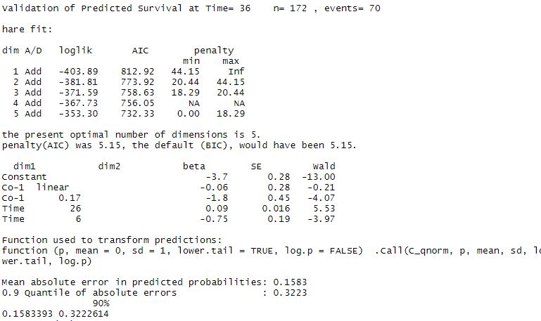
The documentation gives the building blocks but doesn’t put it all together in an obvious way. You either specify a fit object or est.surv and you specify a time point u and the new observed survival time and event indicator as a Surv object in S. If you specify the actual predicted survival probabilities in est.surv they are all for time u. You’ll get a smooth external calibration curve estimate based on hazard regression from the polspline package.

lif · November 18, 2020, 8:37am

Dear Professor, thanks a lot for your reply. I tried with the codes below:

w1<-val.surv(g ,newdata=zzunonsurgical, u=60, S=Surv(zzunonsurgical$TimeToGe,zzunonsurgical$Generalization))
print(w1)
plot(w1)

g represents the lognormal model I developed. Then I get a calibration curve at a specific time point of 60 months with plot (w1), right?

Thank again for your kind help! feng

f2harrell · November 18, 2020, 1:54pm

I think so but it’s fastest to try it yourself. Note I edited your post to format the code.

lif · November 19, 2020, 12:11am

Many many thanks, Professor!

lif · November 19, 2020, 7:28am

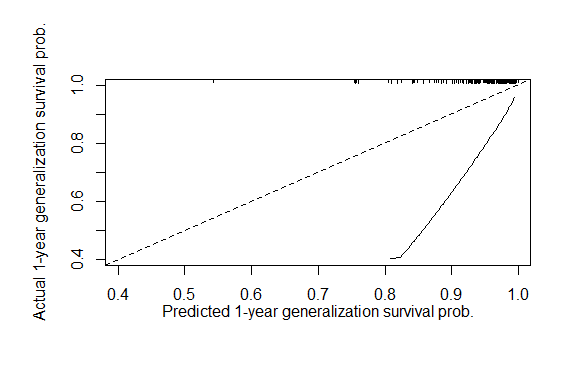
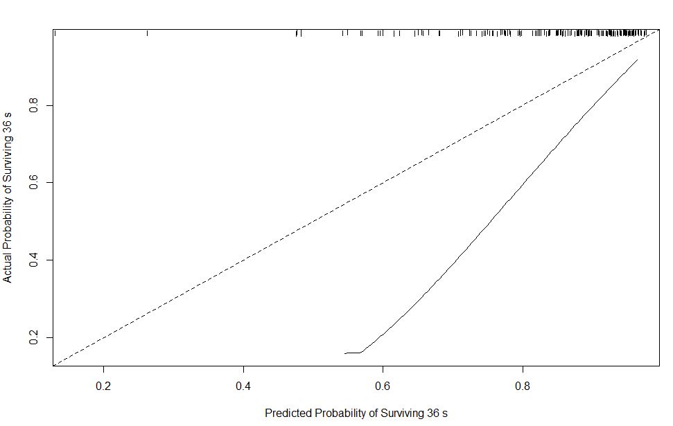
Sorry that I do not know how to edit the codes in the formal way you used. I got a calibration curve which is far from my expectation:

But the c index is acceptable to me,
C Index Dxy S.D. n missing uncensored
7.698844e-01 5.397687e-01 5.563388e-02 1.720000e+02 0.000000e+00 7.000000e+01
Relevant Pairs Concordant Uncertain
1.694800e+04 1.304800e+04 1.230600e+04

For the calculation of the c-index, I used your Hmisc::rcorr.cens function and the codes are as below,
estimates=survest(g,newdata=zzunonsurgical,times=36)$surv
###Determine concordance
surv.obj=with(zzunonsurgical,Surv(TimeToGe,Generalization))
rcorr.cens(x=estimates,S=surv.obj)

Now I still doubt if I am doing it in a right way? May I have your opinion on this please? Thank you!!

f2harrell · November 19, 2020, 12:14pm

Edit you post to include the code to get the calibration curve, and if you haven’t tried it already try using your computed estimates in calling val.surv. Since your validation apparently failed with respect to calibration you can ignore the c-index except to know there is signal in your predictions.

lif · November 19, 2020, 4:02pm

Dear Professor,

Sorry if I am being dim, I re-did the external validation part as far as I understand:

###calibration for external validation
fitlognorm<-psm(Surv(nonsurgical.med$TimeToGe, nonsurgical.med$Generalization)~ MaleGender + AChRValue + AntiMuSKAb + OAID + AgeAtOnset+ SteroidsUse, data = nonsurgical.med, dist = “lognormal”)

g<-update(fitlognorm, x=TRUE, y=TRUE)

estimates=survest(g,newdata=zzunonsurgical,times=36)$surv

w1<-val.surv(g,newdata=zzunonsurgical, S=Surv(zzunonsurgical$TimeToGe, zzunonsurgical$Generalization), est.surv = estimates, u=36)

print(w1)

plot(w1)

Output of print(w1):

Output of plot(w1)

Then I tried to get the c-index:
###Determine concordance
surv.obj=with(zzunonsurgical,Surv(TimeToGe,Generalization))
rcorr.cens(x=estimates,S=surv.obj)

The output reads as below:

If my validation is failed, I will start over again. Thanks a lot for your time, patience and kind help.

f2harrell · November 20, 2020, 12:23pm

I think you did everything right, other than possibly unreasonable linearity assumptions for the covariates. What is the difference in how the training and test datasets were sampled? How many events were in each of the two samples? Why are you using external validation instead of strong internal validation?

One way to check the code is to use val.surv on the training data to make sure you get a (meaningless) perfect calibration plot.

Note that x=TRUE, y=TRUE can be included in psm().

lif · November 21, 2020, 3:16am

Dear Professor, thanks for your reply.

A non-linear effect was not found in any variables included for analyses. I was trying to put knots to continuous variables, but the model’s AIC was smallest when there are no knots added. I found a time-varying effect for the “age” variable, so I chose the lognormal AFT model instead of cox regression.

My colleague collected the training data in a German hospital (n=253, events=113), and then I collected the validating data with the help of one colleague in a Chinese hospital (n=194, events=78). I chose external validation because the two samples are quite different (race, treatment, even diagnostic tests) and the sample size is actually not small given the rarity of the disease.

As you mentioned above, I really got a perfect useless calibration plot using val.surv on the training data. T_T I suppose the model I developed is a failure. One easy solution might be that we combine the two samples, re-develop the model, and then try strong internal validation? But I found this useful paper from Janssen, which showed that “recalibration” methods are recommended to update the model.

BTW, my friends told me that rms::calibrate function can also be used for external validation like this:

set.seed (717)
calv1<-calibrate(fit, cmethod=‘KM’, newdata=external_dataset, m=60, method=‘boot’,u=12,B=400)
calv1
plot(calv1)

But I tried several times in vain. May I have your opinion please? Many thanks.

f2harrell · November 21, 2020, 7:54pm

calibrate only works for internal validation and as you’ll see in the documentation there is no newdata argument.

What you may be observing is a very strong region effect. It is usually better to do a combined analysis and to include region as a variable, hoping that region is in proportional hazards. If using AFT do the stringent residual plot as shown in my RMS course notes to check fit.

lif · November 22, 2020, 8:00am

Dear Professor,

Thanks a lot for guiding me through this. Have a nice weekend!

With best regards
feng

lif · November 22, 2020, 3:57pm

Dear Professor,

I was surfing the internet during the weekend and hope to find some possible solutions for my external validation problem. I found some codes for external validation as below:

s<-Surv(time,event)
fev<- psm(s~ predict(fitlognorm,newdata = validatingdata),x=T,y=T, data = validatingdata, dist=“lognorm”)
cal<- calibrate(fev, cmethod = “KM”, method = “boot”, u=36, m=60,B=100)
plot(cal)

It seems to work for me, but I am a layman for coding and not sure if it makes sense for external validation. Could you please tell me your expression on this?

Thanks a lot and have a good one!
feng

f2harrell · November 23, 2020, 4:19am

That code is not correct. It does internal validatiion on the external sample. You want val.surv for external validation, as we went over earlier.

Steve_Ampah · January 17, 2021, 2:36pm

Hello one and all,
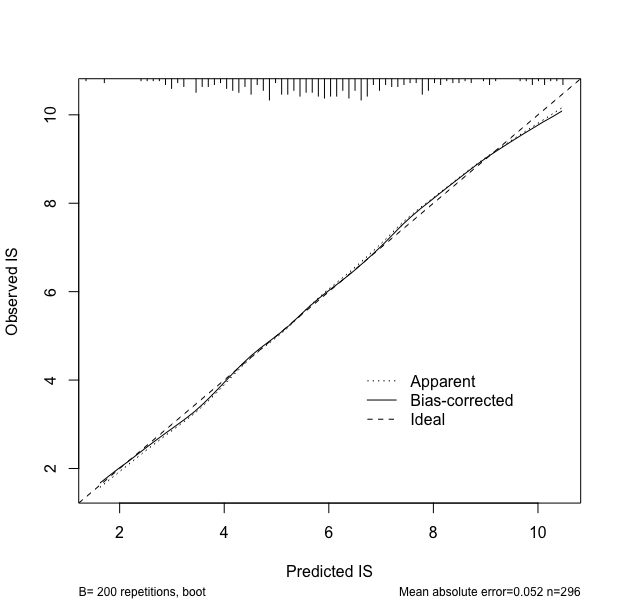
I have a quick question that relates extracting the actual value of the mean absolute error (0.052) on the calibration plot. Is there an easier way of getting this value to be reported in my knitr reproducible report, since source data would be changing I want to avoid cut and paste.

cal=calibrate(mod2,B=200)
plot(cal)

f2harrell · January 17, 2021, 4:32pm

Hello Steve!

That looks like the output from a binary logistic model. Are you sure it’s from a Cox model fit (i.e., from the cph function in the R rms package)?

Questions about RMS are best posted in https://discourse.datamethods.org/t/rms-discussions

Steve_Ampah · January 17, 2021, 5:49pm

It is actually from an ols function, I apologize for asking under Cox model calibration. I searched for calibration and posted it not looking at the topic. Thank you for your quick response.