Comparing 2 biomarkers using restricted cubic splines - how-to, interpretation, model building

Hi everyone,

inspired by the topic started by @kiwiskiNZ - see Troponin, its use and misuse to rule-out and rule-in heart attacks - I had a question as to how you would go about analysing cardiac biomarker data measured at a single time point against two outcome variables:

  1. AMI diagnosis - binary
  2. Death during follow-up

I have been given the advice to enter the cardiac biomarkers log-transformed into a model using restricted cubic splines. After consulting the literature, this makes sense to me - the biomarkers are right-skewed and continuous, and whilst frequently dichotomised, this omits valuable information.
From my interpretation, I could build the following two models:

1) Logistic regression model using @f2harrell’s rms package for the modelling against AMI diagnosis:
Sample data, based on the acath data with some additional biomarker, AMI and FU data:

df <- structure(list(sex = c(0L, 0L, 1L, 1L, 0L, 0L, 0L, 0L, 0L, 0L,
0L, 0L, 1L, 0L, 1L, 0L, 0L, 0L, 0L, 1L), age = c(73L, 68L, 58L,
56L, 41L, 35L, 58L, 81L, 58L, 47L, 66L, 48L, 52L, 67L, 57L, 53L,
62L, 48L, 49L, 59L), cad.dur = c(132L, 85L, 86L, 7L, 15L, 44L,
7L, 2L, 79L, 6L, 8L, 69L, 30L, 48L, 30L, 25L, 87L, 22L, 12L,
3L), choleste = c(268L, 120L, 245L, 269L, 247L, 257L, 168L, 246L,
221L, 272L, 257L, 236L, 240L, 274L, 261L, 273L, 255L, 187L, 252L,
200L), sigdz = c(1L, 1L, 0L, 0L, 1L, 0L, 1L, 1L, 1L, 1L, 1L,
1L, 0L, 1L, 0L, 1L, 1L, 1L, 1L, 1L), tvdlm = c(1L, 1L, 0L, 0L,
0L, 0L, 0L, 1L, 1L, 0L, 0L, 1L, 0L, 1L, 0L, 1L, 0L, 1L, 0L, 0L
), biomarker2 = c(4.48, 33.22, 17.72, 8.74, 9.45, 27.6, 6.78,
9.86, 1055.09, 7.35, 251.15, 19.47, 14.74, 4.53, 5.25, 9.51,
27.42, 8.4, 30.15, 21.66), biomarker1 = c(11.95, 27.28, 8.72,
187.93, 14.61, 91.44, 10.62, 34.58, 110.83, 86.67, 21.41, 12.3,
59.83, 4.75, 14.26, 23.23, 21.49, 79.24, 88.93, 47.01), ami = structure(c(1L,
1L, 1L, 2L, 2L, 1L, 1L, 2L, 1L, 1L, 2L, 1L, 1L, 1L, 1L, 1L, 1L,
1L, 1L, 2L), .Label = c(“0”, “1”), class = “factor”), FU_death = c(1,
0, 0, 1, 0, 0, 0, 0, 1, 0, 0, 0, 0, 0, 0, 1, 0, 0, 0, 0), FU_days = c(647,
562, 617, 563, 663, 21, 548, 617, 535, 593, 648, 468, 589, 589,
630, 744, 556, 581, 654, 452)), row.names = c(“1”, “2”, “4”,
“5”, “8”, “12”, “14”, “15”, “16”, “18”, “19”, “20”, “21”, “22”,
“24”, “25”, “28”, “30”, “31”, “32”), class = “data.frame”)

Fit & plot the model

ddist <- datadist(df)
options(datadist=‘ddist’)
idx_model <- lrm(ami ~ rcs(log(biomarker1), 4), data=df)
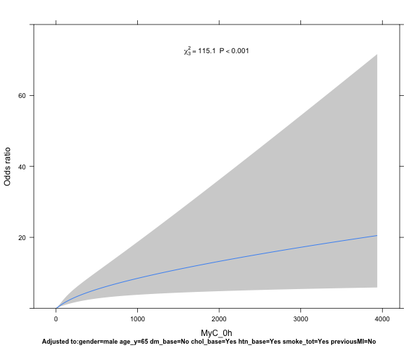
plot(Predict(idx_model, biomarker1, ref.zero=TRUE, fun=exp))

Now this provides a nice plot with the Odds ratio on the y-axis, and the biomarker level on the x-axis. Several questions that play on my mind, however:

  1. How do I best interpret/describe the plot, and extract the Odds ratios at different x-intercepts for a numerical representation of the risk?
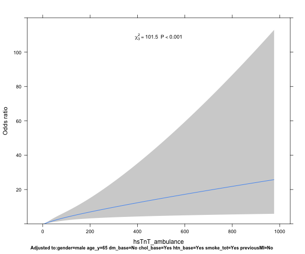
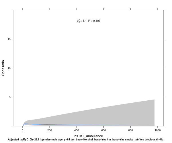
  2. I want to compare the performance of biomarker1 to biomarker2, testing the hypothesis that biomarker1 is better predicting a diagnosis of AMI than biomarker2 - how do I best go about that?
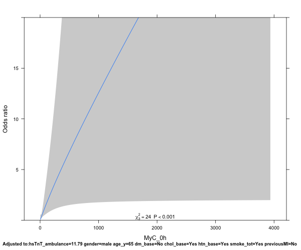
  3. Should I adjust the model for age, gender, known CAD if I know that these factors influence either biomarker concentration, such as here:

idx_model <- lrm(ami ~ rcs(log(biomarker1, 4) + age + sex + choleste + sigdz, data=df)

2) For goal number 2 - analysis of a predictive model, I would suggest the following solution:

fit <- cph(Surv(FU_days, FU_death) ~ rcs(log(biomarker1), 4) + age + sex + choleste + sigdz, data=df)
plot(Predict(fit,biomarker1), xlab=“Biomarker1”, ylab=“Relative Risk”, lty=1, lwd=2)

Again, I would be particularly grateful for your advice on a) interpretation of the results and b) your critique of my approach. Is there a way to compare biomarkers 1+2 in the cox model with cubic splines? Does this make sense?

1 Like

Instead of trying to isolate odds ratios at specific, necessarily arbitrary values, I suggest sticking with the whole curve. The graphic really tells the story, and allows for confidence bands for displaying uncertainty.

As detailed in the maximum likelihood chapter of Regression Modeling Strategies do a likelihood ratio \chi^2 test of whether biomarker 1 adds to biomarker 2 and vice-versa. In each case you are comparing against the “big” inclusive model.

I would adjust for all clinical and demographic variables throughout.

Time to nonfatal MI censored by death is ill-defined. I would do a model for death then a separate model for time to first of (nonfatal MI, death).

1 Like

Nice Tom… I ran your code to understand. Obviously Frank’s the person you should listen too here. Just a thought, though from me - You may find that editors/reviewers want to know the OR at a threshold for the biomarker already in use (eg 99th percentile of troponin). However, with an adjusted model is the graph one of a fictitious group of patients with different biomarker 1 concentrations but all of age 57.5, sex=0 etc? If I understand that correctly (no guarantee!), then I think giving the OR at a threshold is gives too much weight to that fictitious group. Maybe, you could look at a nomogram or shiny app to allow people to play ?
(ps. values can be got from the model from p<-Predict(idx_model, biomarker1, ref.zero=TRUE, fun=exp))

1 Like

Thanks, Frank!

I agree, however, when preparing the data for publication I should still describe the plots to satisfy my reviewers (likely clinicians). I guess I’ll follow your second advice, and do a likelihood χ2 test, and describe the result of that.

I have ordered your book, should be with me tomorrow to check out that chapter. The big inclusive model being one that incorporates all variables including both, the established and the new biomarker?

Excellent point!

Thanks, John! I agree with your sentiment - it is likely I’ll be pushed for an estimate at ‘established’ thresholds. Hence my Q regarding the how-to obtain the OR…the issue, as you point out correctly, is that the other variables would be fixed as per the model (as far as I understand it).

That’s an excellent idea; sadly when I included a dynamic ROC curve recently, the journal showed no interest whatsoever. Should have probably linked to it in the supplement on my own webspace. Will have a think as to how to include a nomogram - any suggestions very welcome!

Static nomograms appear frequently in medical articles. They respect continuous predictors and even allow for interactions. See my course notes and books and even better, Ewout Steyerberg’s book Clinical Prediction Models, for lots of examples.

Thinks like inter-quartile-range odds ratios can be somewhat useful for continuous variables, but they only work well when linearity holds (or at least monotonicity). Ultimately, seeking an odds ratio for discrete levels of a continuous predictor is not very fruitful IMHO.

I don’t think this is a huge issue - at least I’ve not had trouble with it before. What you could do, if there is some value of particular importance a-priori, is drop a vertical (or horizontal) line into the chart and perhaps even add a box with the value at the relevant point into the plot. That way you are not losing any information and the line/box should keep a fussy reviewer happy.

Here is an excellent example of an annotated nomogram.

2 Likes

Nice, thanks Frank! I’ve received your book and started on the Maxiumum likelihood chapter; it’s all become clearer already and I’ve got the three models working. Will update here as soon as I can show some data!

After some experimentation, this is what I’ve come up with - relevant results are included in the code as comments:

dat.models <- select(dat, MyC_0h, hsTnT_ambulance, gender, age_y, dm_base, chol_base, htn_base, smoke_tot, previousMI) # Select all relevant variables
ddist <- datadist(dat.models)
options(datadist=‘ddist’)
ddist$limits[“Adjust to”,“age_y”] <- 65 # Set the age to 65, which is median age in the sample
fit <- update(fit) # make new reference value take effect

idx_model1 <- lrm(AMI ~ rcs(log(MyC_0h), 4) + gender + age_y + dm_base + chol_base + htn_base + smoke_tot + previousMI, data=dat) # Model for biomarker1, using cubic splines with a log-transformed biomarker
idx_model1 # LR chi2 219.03
idx_model2<- lrm(AMI ~ rcs(log(hsTnT_ambulance), 4) + gender + age_y + dm_base + chol_base + htn_base + smoke_tot + previousMI, data=dat) # Model for biomarker2, using cubic splines with a log-transformed biomarker
idx_model2 # LR chi2 201.42
idx_model3<- lrm(AMI ~ rcs(log(MyC_0h), 4) + rcs(log(hsTnT_ambulance), 4) + gender + age_y + dm_base + chol_base + htn_base + smoke_tot + previousMI, data=dat) # Full monty - i.e. all-inclusive model
idx_model3 # LR chi2 226.96

an1 <- anova(idx_model1)
an2 <- anova(idx_model2)
an3 <- anova(idx_model3)

This then allows the calculation of the log likelihood ratio statistic and directly compare the two models (model 1 + 2) against the ‘big’ inclusive model (model 3):

LR = as.numeric(idx_model3$stats[‘Model L.R.’]) # -2 log likelihood ratio statistic for testing joint significance of full set of predictors
LRS.myc = as.numeric(idx_model1$stats[‘Model L.R.’]) # -2 log likelihood ratio statistic for testing importance of subset of predictors of interest
LRS.tnt = as.numeric(idx_model2$stats[‘Model L.R.’])
A = LRS/LR

Formal test of superiority

A.all <- as.numeric(idx_model3$stats[‘Model L.R.’])/as.numeric(idx_model3$stats[‘Model L.R.’])
A.tnt <- as.numeric(idx_model2$stats[‘Model L.R.’])/LR
A.myc <- as.numeric(idx_model1$stats[‘Model L.R.’])/LR
diff.myc <- LR - LRS.myc # What does cTnT add to cMyC = 7.93
diff.tnt <- LR - LRS.tnt # What does cMyC add to cTnT = 25.54

difference being…

diff.both = LRS.myc - LRS.tnt # 17.61

Now, how to plot these models? The following code plots the models, but for the inclusive model I have restricted the yhat to a range of 0-20, as that is most relevant to the question “risk of AMI”:

plot(Predict(idx_model1, MyC_0h, fun=exp), anova=an1, pval=TRUE, ylab=“Odds ratio”)
plot(Predict(idx_model2, hsTnT_ambulance, fun=exp), anova=an2, pval=TRUE, ylab=“Odds ratio”)
plot(Predict(idx_model3, MyC_0h, fun=exp), anova=an3, pval=TRUE, ylab=“Odds ratio”, ylim=c(0,20))
plot(Predict(idx_model3, hsTnT_ambulance, fun=exp), anova=an3, pval=TRUE, ylab=“Odds ratio”, ylim=c(0,20))

This results in the following plots:
Model 1:
model1_oddsratio
Model 2:
model2_oddsratio
Model 3 for biomarker1 (cMyC)
model3_myc_oddsratio
Model 3 for biomarker2 (cTnT)
model3_tnt_oddsratio

Now from my interpretation, both the comparison of the Likelihood ratio test and the plots demonstrate that cMyC adds more to the model than cTnT alone? I’ve also worked on some nomograms, which I’ll add in a separate post. I’d be very grateful for any thoughts on this, as this is pretty new territory for me.

1 Like

As a follow-up, I have created nomograms for the three models - 1) using just cMyC, 2) using hs-cTnT, 3) using both markers.
nomogram1
nomogram2
nomogram3
What I find somewhat counterintuitive is that age seems to have an inverse relationship with risk - similar with some comorbidities such as diabetes (dm_base) or prior MI. In the regression model, one can probably gather that from the negative coefficients, but I’m not certain that I understand why this would be the case? Do the biomarkers explain so much of the model fit that some comorbidities become irrelevant?

Wonder whether @f2harrell or @kiwiskiNZ had any thoughts about this point in particular?

Try using regression to predict age from all the other predictors to learn more about co-linearities. Sometimes it’s also helpful to remove predictors one by one and see how the age effect changes, in the full outcome model.

I’d still like to see what happens if you allow for more action at the lower limit of detection, starting with linear splines.

1 Like

Good point! This is what happens with a simple linear model, using otherwise all other predictors:
lm(formula = age_y ~ rcs(log(MyC_0h), 4) + gender + dm_base +
chol_base + htn_base + smoke_tot + previousMI, data = dat)

Residuals:
    Min      1Q  Median      3Q     Max 
-35.522  -7.230   0.461   7.868  28.762 

Coefficients:
                             Estimate Std. Error t value Pr(>|t|)    
(Intercept)                  30.60685    3.61161   8.475  < 2e-16 ***
rcs(log(MyC_0h), 4)MyC_0h    14.35598    1.69904   8.449  < 2e-16 ***
rcs(log(MyC_0h), 4)MyC_0h'  -50.12907   11.83285  -4.236 2.59e-05 ***
rcs(log(MyC_0h), 4)MyC_0h''  89.91656   26.51431   3.391 0.000737 ***
gendermale                   -5.47067    0.94509  -5.788 1.10e-08 ***
dm_baseYes                   -0.05422    1.18145  -0.046 0.963412    
chol_baseYes                 -1.25164    1.13885  -1.099 0.272151    
htn_baseYes                   6.10119    0.95891   6.363 3.70e-10 ***
smoke_totYes                 -0.66337    0.96778  -0.685 0.493296    
previousMIYes                 3.29272    1.04601   3.148 0.001718 ** 
---
Signif. codes:  0 ‘***’ 0.001 ‘**’ 0.01 ‘*’ 0.05 ‘.’ 0.1 ‘ ’ 1

Residual standard error: 11.38 on 664 degrees of freedom
  (102 observations deleted due to missingness)
Multiple R-squared:  0.3556,	Adjusted R-squared:  0.3468 
F-statistic: 40.71 on 9 and 664 DF,  p-value: < 2.2e-16

And with all biomarkers included:
lm(formula = age_y ~ rcs(log(MyC_0h), 4) + rcs(log(hsTnT_ambulance),
4) + gender + dm_base + chol_base + htn_base + smoke_tot +
previousMI, data = dat)

Residuals:
    Min      1Q  Median      3Q     Max 
-36.443  -6.759   0.945   7.615  24.284 

Coefficients:
                                              Estimate Std. Error t value Pr(>|t|)    
(Intercept)                                    17.5463     4.1076   4.272 2.23e-05 ***
rcs(log(MyC_0h), 4)MyC_0h                       7.8388     1.9343   4.053 5.67e-05 ***
rcs(log(MyC_0h), 4)MyC_0h'                    -49.5402    13.9897  -3.541 0.000426 ***
rcs(log(MyC_0h), 4)MyC_0h''                    98.2164    32.1246   3.057 0.002323 ** 
rcs(log(hsTnT_ambulance), 4)hsTnT_ambulance    14.9981     2.6524   5.655 2.33e-08 ***
rcs(log(hsTnT_ambulance), 4)hsTnT_ambulance'  -22.9552    18.6805  -1.229 0.219573    
rcs(log(hsTnT_ambulance), 4)hsTnT_ambulance''  27.9816    41.9263   0.667 0.504751    
gendermale                                     -6.4153     0.8952  -7.166 2.07e-12 ***
dm_baseYes                                     -1.2663     1.1142  -1.136 0.256191    
chol_baseYes                                   -0.9990     1.0682  -0.935 0.350014    
htn_baseYes                                     4.8947     0.9060   5.403 9.17e-08 ***
smoke_totYes                                   -0.8572     0.9071  -0.945 0.345005    
previousMIYes                                   3.0480     0.9798   3.111 0.001946 ** 
---
Signif. codes:  0 ‘***’ 0.001 ‘**’ 0.01 ‘*’ 0.05 ‘.’ 0.1 ‘ ’ 1

Residual standard error: 10.65 on 661 degrees of freedom
  (102 observations deleted due to missingness)
Multiple R-squared:  0.4384,	Adjusted R-squared:  0.4282 
F-statistic: 43.01 on 12 and 661 DF,  p-value: < 2.2e-16

I guess the high estimates of all the biomarkers tell me what you’ve been suggesting.

I thought we had included linear splines for the biomarkers (cMyC, hsTnT) by using rcs in the lrm function call?

rcs is restricted cubic spline. It is our best default method when smoothness is expected. When there is a possible discontinuity as with lower detection limits (e.g. there may be a jump in risk when you get a tiny bit above the limit) you have to put a lot of knots near the discontinuity to model it properly. A linear spline has only a zero-order discontinuity restriction (line segments must meet each other) and allows for a huge jump in slope exactly at a knot. So as I mentioned earlier, the most general way to model this is to have an indicator for being at or below the detection limit then have a restricted cubic spline for the rest, and to combine all those terms to get prediction-as-a-whole. But an easier first step is to fit a linear spline with knots at values such as the 0.01 quantile of values above the detection limit, and the 0.25 0.5 0.75 quantiles of the above-limit values.

1 Like

Obviously Frank’s responded to this Tom. Just from a physiological perspective, have you plasma or serum creatinine you could substitute for Age?

When using the R rms package, use the ols function for linear models to get better formatting of output, and more informative stats.

Thanks! I have removed predictors as you’ve suggested, both in the model predicting age and the model predicting AMI:

Frequencies of Missing Values Due to Each Variable
     age_y     MyC_0h     gender    dm_base  chol_base   htn_base  smoke_tot previousMI 
         0          0          0          0          0          0        102          0 

Linear Regression Model
 
 ols(formula = age_y ~ rcs(log(MyC_0h), 4) + gender + dm_base + 
     chol_base + htn_base + smoke_tot + previousMI, data = dat)
 
 
                 Model Likelihood     Discrimination    
                    Ratio Test           Indexes        
 Obs      674    LR chi2    296.16    R2       0.356    
 sigma11.3820    d.f.            9    R2 adj   0.347    
 d.f.     664    Pr(> chi2) 0.0000    g        9.377    
 
 Residuals
 
     Min      1Q  Median      3Q     Max 
 -35.522  -7.230   0.461   7.868  28.762 
 
 
                Coef     S.E.    t     Pr(>|t|)
 Intercept       30.6068  3.6116  8.47 <0.0001 
 MyC_0h          14.3560  1.6990  8.45 <0.0001 
 MyC_0h'        -50.1291 11.8329 -4.24 <0.0001 
 MyC_0h''        89.9166 26.5143  3.39 0.0007  
 gender=male     -5.4707  0.9451 -5.79 <0.0001 
 dm_base=Yes     -0.0542  1.1814 -0.05 0.9634  
 chol_base=Yes   -1.2516  1.1388 -1.10 0.2722  
 htn_base=Yes     6.1012  0.9589  6.36 <0.0001 
 smoke_tot=Yes   -0.6634  0.9678 -0.69 0.4933  
 previousMI=Yes   3.2927  1.0460  3.15 0.0017  

Then without the smoking variable (note that the model above would only draw on 674 observations as 102 patients had a missing smoking status), and after some experimenting the model with the highest LR chi2:

Linear Regression Model
 
 ols(formula = age_y ~ rcs(log(MyC_0h), 4) + gender + dm_base + 
     chol_base + htn_base + previousMI, data = dat)
 
                 Model Likelihood     Discrimination    
                    Ratio Test           Indexes        
 Obs      776    LR chi2    369.16    R2       0.379    
 sigma11.5181    d.f.            8    R2 adj   0.372    
 d.f.     767    Pr(> chi2) 0.0000    g        9.957    
 
 Residuals
 
      Min       1Q   Median       3Q      Max 
 -37.6950  -7.2712   0.6042   7.8979  28.9518 
 
 
                Coef     S.E.    t     Pr(>|t|)
 Intercept       30.0435  3.4406  8.73 <0.0001 
 MyC_0h          14.4039  1.6076  8.96 <0.0001 
 MyC_0h'        -44.7188 11.0554 -4.04 <0.0001 
 MyC_0h''        76.3353 24.6210  3.10 0.0020  
 gender=male     -5.7163  0.8704 -6.57 <0.0001 
 dm_base=Yes      0.6130  1.0909  0.56 0.5743  
 chol_base=Yes   -1.6497  1.0645 -1.55 0.1216  
 htn_base=Yes     5.6333  0.9078  6.21 <0.0001 
 previousMI=Yes   3.5624  0.9681  3.68 0.0002

Yes, I do! Let me have a look and get back to you on this.

Good. You could also play with estimated GFR (eGFR). Use the CKD-EPI formula (not MDRD) and drop Age and Sex from the regression equation. eGFR equations are not brilliant - but if the question is around the influence of renal function on troponin/myC, then it may be worth a look (maybe look at a linear regression of eGFR with biomarkers?). Of course, the assumption is that when the creatinine was measured the true GFR was stable (I’m not convinced about that - but that’s a topic for another day).