I have gone about solving the regression in the following manner:
Determine quantiles (0.01, 0.25, 0.5, 0.75) for each biomarker above the LoD
Fit linear splines with above quantiles - however, I got an error when trying to fit the model using lrm.fit with a 1% quantile above the LoD. It would only compute at 0.12 quantile - maybe I’m overlooking something?
Build regression model with all relevant risk factors, and as suggested by @kiwiskiNZ, including the CKD-EPI formula, thus omitting age & gender from the regression equation.
Frequencies of Missing Values Due to Each Variable
            AMI          MyC_0h hsTnT_ambulance         gfr_epi         dm_base
              0               0               0              84               0
      chol_base        htn_base      previousMI
              0               0               0

Logistic Regression Model

 lrm(formula = AMI ~ lsp(MyC_0h, myc.quant) + lsp(hsTnT_ambulance,
     tnt.quant) + gfr_epi + dm_base + chol_base + htn_base + previousMI,
     data = dat)


                        Model Likelihood     Discrimination    Rank Discrim.
                           Ratio Test           Indexes           Indexes
 Obs            692    LR chi2     256.87    R2       0.469    C       0.866
  0             532    d.f.            15    g        2.827    Dxy     0.732
  1             160    Pr(> chi2) <0.0001    gr      16.897    gamma   0.732
 max |deriv| 0.0001                          gp       0.263    tau-a   0.261
                                             Brier    0.109

                     Coef     S.E.    Wald Z Pr(>|Z|)
 Intercept           -22.0606 10.4984 -2.10  0.0356
 MyC_0h                1.9825  1.4746  1.34  0.1788
 MyC_0h'              -2.2639  1.5749 -1.44  0.1506
 MyC_0h''              0.3488  0.2605  1.34  0.1806
 MyC_0h'''            -0.0350  0.0532 -0.66  0.5110
 MyC_0h''''           -0.0321  0.0105 -3.05  0.0023
 hsTnT_ambulance       0.5085  0.4831  1.05  0.2925
 hsTnT_ambulance'     -0.4553  1.1983 -0.38  0.7039
 hsTnT_ambulance''     0.1270  0.8750  0.15  0.8846
 hsTnT_ambulance'''   -0.1716  0.1021 -1.68  0.0929
 hsTnT_ambulance''''  -0.0044  0.0271 -0.16  0.8723
 gfr_epi               0.0281  0.0057  4.92  <0.0001
 dm_base=Yes          -0.9719  0.3163 -3.07  0.0021
 chol_base=Yes         0.3064  0.3181  0.96  0.3354
 htn_base=Yes          0.0979  0.2494  0.39  0.6948
 previousMI=Yes       -0.0445  0.2483 -0.18  0.8578

Frequencies of Missing Values Due to Each Variable
       AMI     MyC_0h    gfr_epi    dm_base  chol_base   htn_base previousMI
         0          0         84          0          0          0          0

Logistic Regression Model

 lrm(formula = AMI ~ lsp(MyC_0h, myc.quant) + gfr_epi + dm_base +
     chol_base + htn_base + previousMI, data = dat)


                       Model Likelihood     Discrimination    Rank Discrim.
                          Ratio Test           Indexes           Indexes
 Obs           692    LR chi2     242.72    R2       0.448    C       0.856
  0            532    d.f.            10    g        2.504    Dxy     0.711
  1            160    Pr(> chi2) <0.0001    gr      12.231    gamma   0.711
 max |deriv| 3e-05                          gp       0.257    tau-a   0.253
                                            Brier    0.112

                Coef     S.E.   Wald Z Pr(>|Z|)
 Intercept      -18.4166 9.6059 -1.92  0.0552
 MyC_0h           1.9705 1.4042  1.40  0.1605
 MyC_0h'         -2.0841 1.4968 -1.39  0.1638
 MyC_0h''         0.2164 0.2467  0.88  0.3803
 MyC_0h'''       -0.0598 0.0502 -1.19  0.2334
 MyC_0h''''      -0.0420 0.0082 -5.13  <0.0001
 gfr_epi          0.0233 0.0052  4.44  <0.0001
 dm_base=Yes     -0.8962 0.3145 -2.85  0.0044
 chol_base=Yes    0.2060 0.3070  0.67  0.5023
 htn_base=Yes     0.1628 0.2453  0.66  0.5069
 previousMI=Yes  -0.0411 0.2472 -0.17  0.8678

Frequencies of Missing Values Due to Each Variable
            AMI hsTnT_ambulance         gfr_epi         dm_base       chol_base
              0               0              84               0               0
       htn_base      previousMI
              0               0

Logistic Regression Model

 lrm(formula = AMI ~ lsp(hsTnT_ambulance, tnt.quant) + gfr_epi +
     dm_base + chol_base + htn_base + previousMI, data = dat)


                       Model Likelihood     Discrimination    Rank Discrim.
                          Ratio Test           Indexes           Indexes
 Obs           692    LR chi2     231.35    R2       0.430    C       0.849
  0            532    d.f.            10    g        2.275    Dxy     0.698
  1            160    Pr(> chi2) <0.0001    gr       9.724    gamma   0.698
 max |deriv| 0.002                          gp       0.250    tau-a   0.248
                                            Brier    0.116

                     Coef    S.E.   Wald Z Pr(>|Z|)
 Intercept           -9.7911 2.6558 -3.69  0.0002
 hsTnT_ambulance      0.6282 0.4268  1.47  0.1410
 hsTnT_ambulance'    -0.4979 1.0905 -0.46  0.6480
 hsTnT_ambulance''    0.1676 0.8135  0.21  0.8368
 hsTnT_ambulance'''  -0.2298 0.0947 -2.43  0.0152
 hsTnT_ambulance'''' -0.0616 0.0220 -2.81  0.0050
 gfr_epi              0.0283 0.0055  5.11  <0.0001
 dm_base=Yes         -1.0309 0.3104 -3.32  0.0009
 chol_base=Yes        0.3356 0.3064  1.10  0.2734
 htn_base=Yes         0.0565 0.2419  0.23  0.8153
 previousMI=Yes       0.0463 0.2425  0.19  0.8486
I’m not convinced that the linear spline fits better than the restricted cubic spline quoted above? In fact, the LR chi2 is 259, R2 0.473 and C index 0.865 for the all-inclusive model using rcs, which I think points to a better model fit?
Need to play a little more on regression of eGFR with biomarkers - not convinced I’ve got a conclusive answer yet, but you can see the implementation of eGFR in the above analysis John!
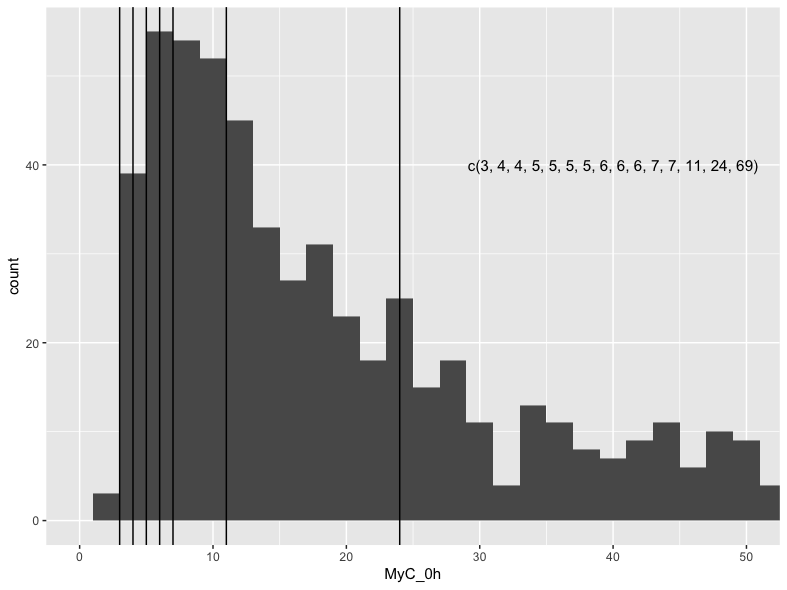
The cubic spline model is probably better. I just want to make sure a discontinuity isn’t needed near the threshold (detection limit). Not clear why the linear spline wouldn’t fit with the first knot closer to the limit. May be good to show us a high-resolution histogram of the measurements along with reference lines showing all the quantiles that were considered.
You must have more ties in the data than I suspected, which would cause the difficulty. But the histograms are not high resolution enough. Just show the output of table() perhaps.
I must be missing something obvious but I can’t see why putting a knot at 5.37 for the linear spline wouldn’t work, and this would effectively estimate the separate effect of being below the LOD. If that doesn’t work, then maybe at 6. Make sure the values below LOD are coded as LOD and not zero. Can also fit a restricted cubic spline with an extra knot just above 5.37 to allow complexity near LOD.
All patients have a biomarker result above the LOD (for cMyC). I have trialled different cut-offs/knots now, the closest I can get to 5.37 is with a knot at 8 - not sure either why this might be? Also, 8 seems to be too close to 11 (0.25 quantile), so I had to adjust the second knot to 12 so that it can fit the model. This would be output from the cMyC-only model:
lrm(AMI ~ lsp(MyC_0h, c(8, 12, 24, 69)) + gfr_epi + dm_base + chol_base + htn_base + previousMI, data=dat) # cMyC model

Frequencies of Missing Values Due to Each Variable
       AMI     MyC_0h    gfr_epi    dm_base  chol_base   htn_base previousMI
         0          0         84          0          0          0          0

Logistic Regression Model

 lrm(formula = AMI ~ lsp(MyC_0h, c(8, 12, 24, 69)) + gfr_epi +
     dm_base + chol_base + htn_base + previousMI, data = dat)


                       Model Likelihood     Discrimination    Rank Discrim.
                          Ratio Test           Indexes           Indexes
 Obs           692    LR chi2     242.18    R2       0.447    C       0.857
  0            532    d.f.            10    g        2.242    Dxy     0.713
  1            160    Pr(> chi2) <0.0001    gr       9.416    gamma   0.713
 max |deriv| 3e-06                          gp       0.257    tau-a   0.254
                                            Brier    0.112

                Coef     S.E.   Wald Z Pr(>|Z|)
 Intercept      -12.1604 3.9805 -3.05  0.0023
 MyC_0h           0.9627 0.5255  1.83  0.0670
 MyC_0h'         -1.1365 0.6423 -1.77  0.0768
 MyC_0h''         0.2934 0.2401  1.22  0.2217
 MyC_0h'''       -0.0773 0.0559 -1.38  0.1662
 MyC_0h''''      -0.0413 0.0082 -5.02  <0.0001
 gfr_epi          0.0233 0.0052  4.45  <0.0001
 dm_base=Yes     -0.8958 0.3146 -2.85  0.0044
 chol_base=Yes    0.2116 0.3070  0.69  0.4907
 htn_base=Yes     0.1616 0.2454  0.66  0.5103
 previousMI=Yes  -0.0417 0.2474 -0.17  0.8662
So I’m not sure about that either. One would think there are enough cases at that knot?
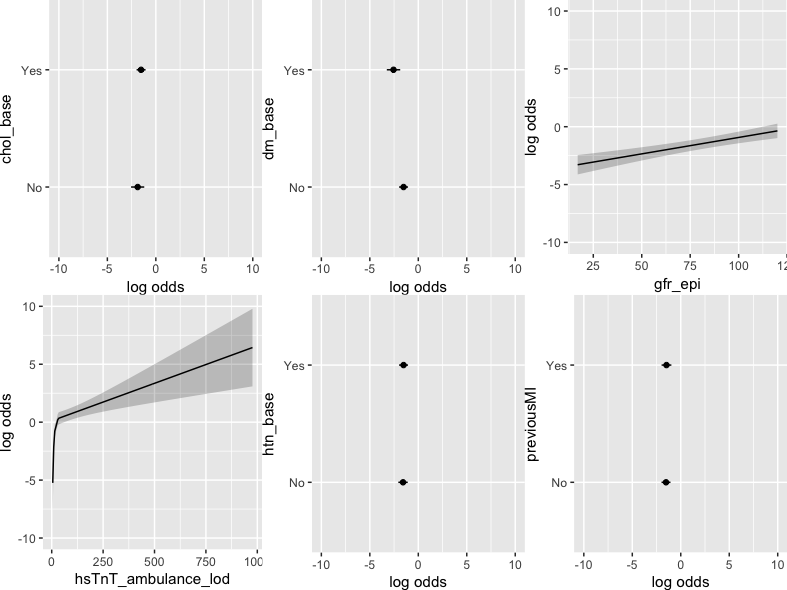
I hadn’t caught that. None of the complexities apply for that marker and ordinary knot locations can be used. Show partial effect plot for the linear spline for the one that had values below LOD, e.g. ggplot(Predict(...)).
Excellent, one aspect solved I take it rcs(MyC_0h, 4) for restricted cubic spline with 4 knots is adequate?
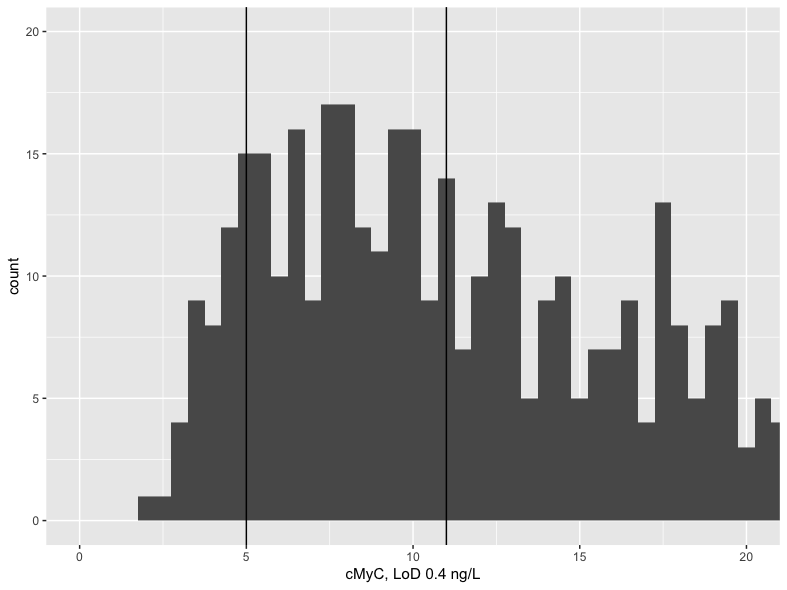
cTnT has values below LOD (5 ng/L) which I’ve re-coded to 4.99. The quantiles you suggested come out at 5, 8, 14, 31. The lsp model computes at a first knot of 5.5:
> mod3 <- lrm(AMI ~ lsp(hsTnT_ambulance, c(5.5, 8, 14, 31)) + gfr_epi + dm_base + chol_base + htn_base + previousMI, data=dat) # hs-cTnT model
> mod3
Frequencies of Missing Values Due to Each Variable
            AMI hsTnT_ambulance         gfr_epi         dm_base       chol_base
              0               0              84               0               0
       htn_base      previousMI
              0               0

Logistic Regression Model

 lrm(formula = AMI ~ lsp(hsTnT_ambulance, c(5.5, 8, 14, 31)) +
     gfr_epi + dm_base + chol_base + htn_base + previousMI, data = dat)


                       Model Likelihood     Discrimination    Rank Discrim.
                          Ratio Test           Indexes           Indexes
 Obs           692    LR chi2     234.08    R2       0.434    C       0.849
  0            532    d.f.            10    g        2.668    Dxy     0.699
  1            160    Pr(> chi2) <0.0001    gr      14.407    gamma   0.699
 max |deriv| 7e-05                          gp       0.251    tau-a   0.249
                                            Brier    0.116

                     Coef     S.E.    Wald Z Pr(>|Z|)
 Intercept           -20.9423 11.7865 -1.78  0.0756
 hsTnT_ambulance       2.8236  2.1877  1.29  0.1968
 hsTnT_ambulance'     -2.8094  2.3351 -1.20  0.2289
 hsTnT_ambulance''     0.3012  0.3781  0.80  0.4257
 hsTnT_ambulance'''   -0.2481  0.0926 -2.68  0.0074
 hsTnT_ambulance''''  -0.0608  0.0219 -2.77  0.0056
 gfr_epi               0.0285  0.0056  5.13  <0.0001
 dm_base=Yes          -1.0369  0.3103 -3.34  0.0008
 chol_base=Yes         0.3546  0.3062  1.16  0.2469
 htn_base=Yes          0.0543  0.2418  0.22  0.8222
 previousMI=Yes        0.0454  0.2427  0.19  0.8515
Very informative. Sometimes we backup spline analyses with nonparametric regression (e.g., loess) but loess doesn’t work perfectly when Y is binary even if you turn off outlier detection.
I’ve been following this discussion about placement of knots. I too have noticed some difficulty in the past. I wonder if the knots are placed in such a way that either below the lowest, or between two knots the problem occurs because there are too few patients with the outcome of interest?
Very possible, John! Of course, we know that AMI is extremely unlikely below certain concentrations, and we might only find 1 or 2 cases of AMI below, say, 20 ng/L (of cTnT). This cohort consists also of very-early presenters, hence cTnT is very likely still in the early phases of release.
// edit: Although, I’m not sure whether the splines care about the number of cases at/below each knot? It would just be my assumption that this could influence whether a model works or not…
Why would you consider creatinine (or eGFR) as a substitute for age?
A-priori, I would assume that while creatinine may have a relationship with age, both age and creatinine likely also have an independent relationship with risk for AMI. Personally I would try a model including both terms.
@tomkaier regarding splines - perhaps some of the other continuous variables also have nonlinear relationships with AMI? I would expect eGFR to have a non-linear relationship for example. Alternatively, perhaps there is an interaction between troponin and eGFR (given that worse eGFR will effect the half-life of elimination of troponin I would again expect such an interaction).
I guess John’s @kiwiskiNZ thought was that the GFR-epi formula incorporates age, gender and race and may be omitted in the logistic regression. In fact, GFR makes the model fit worse. In comparison, a model incorporating all cardiovascular risk factors, smoking status, gender, age and creatinine plus cardiac biomarkers (rcs for cMyC, lsp for cTnT) results in a R2 0.499 and C 0.879. If you run a fast backward variable selection (using AIC as the stopping rule) on this, the factors in the final model are cMyC, creatine and gender. This model yields an R2 0.447, C 0.862, but is obviously way more parsimonious and easily translated into a nomogram.
Good point! Splines haven’t improved the fit dramatically when used for creatinine. Looks fairly evenly distributed on histogram too.
Ah right yes I did not think of that, although in general its better to include each individual term over composite terms if you can.
Did you try the interaction model ? I would do that before adding splines. So do something like:
Model1: AMI ~ cMyc + creatintine + other_vars
Model2: AMI ~ cMyc * creatintine + other_vars
lrt(Model1, Model2)