Determining post-test probability of Covid-19

I did this for myself this weekend. I could not find anything online that provided the plot I do here. I wanted to post this somewhere in case someone else was in a similar situation, but I hoped to run it by the folks here for feedback first.

I included the Rmd file below, but here is the plot for convenience.


title: “Determining post-test probability of Covid-19”
output:
pdf_document: default
html_document: default

knitr::opts_chunk$set(echo = TRUE)

Caution: I use standard methods, but this is quickly put together – use at your own risk. If you find any mistakes, let me know and I will correct them. There are calculators online, but it is not easy to find the plot below. Hopefully it might help someone else in a similar situation.

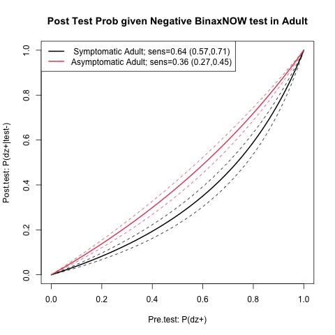
In summary, it would be useful to quickly be able to assess post-test covid-19 risk (using available studies). For example, here, in an asymptomatic adult with a negative BinaxNOW rapid antigen test. This could instruct how one goes about the next week, etc.

Per current guidelines, if you are exposed, vaccinated and have a negative test you can go about life fairly normally. However, I had a clinic this week with immunocompromised patients, and I wanted to be sure that I would not potentially expose anyone (I am just a trainee, so I am nonessential). So, I wanted the most actionable risk estimate I could get. So, I hoped to find the probability that I have a coronavirus infection given that I test negative and the probability that I have a coronavirus infection if I test negative twice.

These rapid tests are sometimes designed such that a positive result implies that the true status is positive, but a negative result might be a false negative. This is essentially what is said in the test kit.
It is however sort of difficult to interpret this. This means that there are few false positives, or high specificity, and sometimes false negatives, or lower sensitivity. This is also sort of difficult to interpret. I hope here to give you a result that is easier to interpret.

We want to know the probability that someone has the disease given a test, which is is more intuitive. It is possible to get this, but you have to calculate using Bayes rule. I will do the calculations here for you.

The issue is that any post test probability (posterior) depends on a pre-test probability (prior). Sometimes this is “prevalence”. However, your prior might be different than the prevalence;
you may stay in more, for example, or have had contact recently with an infected individual.

For a large prior, we see that a negative test result is not very conclusive. Doing serial testing and getting 2 negative results is more conclusive, but of course it depends on the original prior.

We could of course say that the prior is too difficult to determine and throw our hands up, but in doing so we are implicitly acting according to some prior, and just choosing not to discuss it further. From a decision analysis standpoint, attending a clinic with immunocompromised patients could have great cost, so it is worth trying to be explicit about how we are making this decision. Here, I will show post test probabilities for a variety of priors.

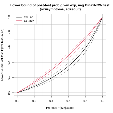
Note that the numbers below are not applicable to symptomatic adults or children. The studies I found stratify by symptoms and age and therefore these grouops have different sensitivities and specificities. The code could be changed though for that if needed.

I checked the number against the PPV/NPV for one of the studies listed below, and it was close
but not identical

I also checked my Bayes rule numbers against the calculator (Diagnostic Test Calculator), written by Alan Schwartz alansz@uic.edu, and our values matched.

Update: (showed work)

The posterior is

P(dz+|test-)=\frac{P(test-|dz+)}{P(test-)}P(dz+)=\frac{1-P(test+|dz+)}{P(test-|dz-)P(dz-)+P(test-|dz+)P(dz+)}P(dz+).

Note that

Sensitivity = P(test+|dz+),
Specificity = P(test-|dz-).

Hence,
\frac{1-P(test+|dz+)}{P(test-|dz-)P(dz-)+P(test-|dz+)P(dz+)}=\frac{1-sens}{spec*(1-P(dz+))+(1-sens)*P(dz+)}

is the likelihood ratio in terms of quantities that we can glean from the studies.

like.rat=function(sens,spec,pretest){(1-sens)/((1-sens)*pretest+(spec)*(1-pretest))}
pretest=0.2

The posterior probability of having the disease given a negative test result is (likelihood ratio) * prior.

post.test.prob = function(sens,spec,pretest){
  like.rat(sens=sens,spec=spec,pretest=pretest)*pretest
}

Since the prior/pre-test probability is subjective, we can use `R’ to plot the post test probability over a range.

pre.tests = seq(0,1,0.01)
get.post.tests = function(sens,spec,pretests){
post.tests = c()
for(i in 1:length(pre.tests)){
  post.tests[i]=post.test.prob(sens=sens,spec=spec,pretest=pre.tests[i])
}
post.tests
}

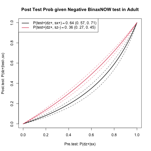
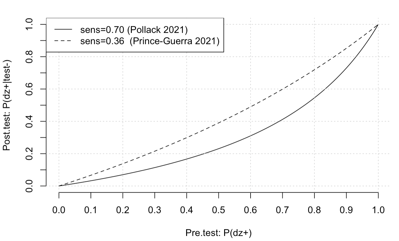
I will compute two different post-test probability lines, one for each study [1,2], using the reported sensitivity and specificity for asymptomatic adults. Each study has different sensitivity, but similar specificity. Hence I will label the study by the sensitivity.

post.tests.6=get.post.tests(sens=0.70,spec=1,pretests)
plot(pre.tests,post.tests.6,type='l',xlab="Pre.test: P(dz+)",ylab="Post.test: P(dz+|test-)",lty=1,axes=FALSE)
axis(side = 1, at = seq(0,1,0.1))
axis(side = 2, at = seq(0,1,0.1))
grid()
post.tests.36=get.post.tests(sens=0.36,spec=1,pretests)
lines(pre.tests,post.tests.36,lty=2)
legend("topleft",c("sens=0.70 (Pollack 2021)","sens=0.36  (Prince-Guerra 2021)"),lty=c(1,2))

So, suppose that I am really not sure. I was in proximity to someone with the disease. Then maybe my pretest probability is a coin flip, 0.5. We trace this up to between the tests to get a post test probability of about 0.3 (very rough). You can get more exact number with the function above, but the main point is that the post test probability, even with a negative test, is not very low. So, given one test, with the prior of 0.5, it is probably best not to go out too much, and definitely risky to go to a clinic with immunocompromised patients, especially if you are not essential.

If I take a second test, I can update my old pre test probability to be my new post test probability. In this case, I start around 0.3 on the x-axis and go to about 0.1. Still, this is a sizeable risk. You can see however why serial testing is better than one test.

In general, I decided not to attend the clinic, and also to switch a meeting I had this week to Zoom.

If you think that the probability of disease given a negative result is useful, you might also be interested in [3].

References

[1] Prince-Guerra JL, Almendares O, Nolen LD, Gunn JKL, Dale AP, Buono SA, Deutsch-Feldman M, Suppiah S, Hao L, Zeng Y, Stevens VA, Knipe K, Pompey J, Atherstone C, Bui DP, Powell T, Tamin A, Harcourt JL, Shewmaker PL, Medrzycki M, Wong P, Jain S, Tejada-Strop A, Rogers S, Emery B, Wang H, Petway M, Bohannon C, Folster JM, MacNeil A, Salerno R, Kuhnert-Tallman W, Tate JE, Thornburg NJ, Kirking HL, Sheiban K, Kudrna J, Cullen T, Komatsu KK, Villanueva JM, Rose DA, Neatherlin JC, Anderson M, Rota PA, Honein MA, Bower WA. Evaluation of Abbott BinaxNOW Rapid Antigen Test for SARS-CoV-2 Infection at Two Community-Based Testing Sites - Pima County, Arizona, November 3-17, 2020. MMWR Morb Mortal Wkly Rep. 2021 Jan 22;70(3):100-105. doi: 10.15585/mmwr.mm7003e3. Erratum in: MMWR Morb Mortal Wkly Rep. 2021 Jan 29;70(4):144. PMID: 33476316; PMCID: PMC7821766.

[2] Pollock NR, Jacobs JR, Tran K, Cranston AE, Smith S, O’Kane CY, Roady TJ, Moran A, Scarry A, Carroll M, Volinsky L, Perez G, Patel P, Gabriel S, Lennon NJ, Madoff LC, Brown C, Smole SC. Performance and Implementation Evaluation of the Abbott BinaxNOW Rapid Antigen Test in a High-Throughput Drive-Through Community Testing Site in Massachusetts. J Clin Microbiol. 2021 Apr 20;59(5):e00083-21. doi: 10.1128/JCM.00083-21. PMID: 33622768; PMCID: PMC8091851.

[3] Moons, Karel GM, and Frank E. Harrell. “Sensitivity and specificity should be de-emphasized in diagnostic accuracy studies.” Academic radiology 10.6 (2003): 670-672. http://hbiostat.org/papers/feh/moons.radiology.pdf

4 Likes

Is it easy for you to add more tick-marks on the x-axis and the y-axis so that estimating the post-test probability from the pre-test probability is a bit more precise and your examples easier to follow?

I like the idea of an individual thinking about their hypothetical “personal” pre-test prior based on their exposure situation (e.g., just got off an airplane, got coughed on by someone without a mask, haven’t left the house in 14 days) with decisions about personal subsequent behavior based on the estimated post-test probability given a negative test (e.g., stay isolated for 7 days, do the meeting using ZOOM, roam freely).

2 Likes

Isnt your likelihood ratio calculation FNR/total negative tests expected rather than FNR/TNR? Also there is notable uncertainty in the sensitivity estimates from the Pollock paper for asymptomatic adults 70.2 (56.6–81.6).

1 Like

Done, thank you!

Yes, I agree! I think you have worded it better than I did

I have included my alegbra for the LR above in an edit. I am not sure if that will answer, if not I can try another way

Yes, that is true. I guess I should add some type of intervals around the lines

I have fixed some things - it turns out I had actually mixed up some of the numbers from the different studies before (the lines were from symptomatic adults and asymptomatic adults in one study, not for asymptomatic adults over 2 studies). I sort of liked this more, so I set aside Pollock, and remade the plots only using numbers from Prince-Guerra 2021, this time with CI as suggested. I wish I could edit the original post to get the incorrect image off the top.

I realize the final post test from this type of procedure might not be too accurate - there are issues with estimates like sensitivity in the first place. However, it is all I can see that there is to go by in this kind of situation.

I guess (I hope) that at least looking at this plot is better than just getting a negative result and then interpreting it as a negative disease (?). The thing is that these rapid tests have good specificity, but the sensitivity is generally poor.

post.test

1 Like

In my opinion, you deserve a compliment for your effort to keep improving the “tool” using the best available data (which appears to be not so good). Your work continues to draw attention to the idea of a “personal” prior, which could help a person to decide what decisions they might make about their behavior in light of the data (and uncertainties). The data will probably get better (but not soon).

While I sympathize with your desire to “get rid of” the incorrect image in the original post, I see this “string” of posts as showcasing “science in action”

2 Likes

Thank you again - yes, point taken. I wish I had been more careful the first time, but this is sort of on my back burner - I come back to it actually every time someone I know has a negative result from a rapid antigen, then end up finding out they were in fact positive, usually with negative consequences for them (twice now!)

Thinking more about this. Actually, we can write this all as conditional on symptom status. Then, we see more clearly that we have essentially a binary random variable for symptoms (which is not ideal). Also, I had written sens= in the legend. It should be approximate. I also just try to get rid of terminology. Here is a better summary

A positive BinaxNOW Covid-19 Antigen selfTEST is a good indicator that covid-19 is present. A negative result, however, is less conclusive [1]. How to therefore proceed in light of a negative test?

Here are some rough (getting less rough) thoughts. From Prince-Guerra et al (2021) [2], P(test+|dz+,sx=1) \approx 0.64 (0.57,0.71) and P(test+|dz+,sx=0) \approx 0.36 (0.27,0.45). Also, P(dz-|test-,sx=0)\approx 1 (1,1) and P(dz-|test-,sx=1)\approx 1 (1,1).

Now,

P(dz+|test-,sx)=\frac{P(test-|dz+,sx)}{P(test-|sx)}P(dz+|sx) =\frac{1-P(test+|dz+,sx)}{P(test-|dz-,sx)P(dz-|sx)+P(test-|dz+,sx)P(dz+|sx)}P(dz+|sx).

Hence (code here).

post.test

Ideally, studies would model P(dz+|test-,sx,age,sex,\dots) directly, but then we also lose some flexibility, since if I want to customize my pretest, it is difficult to do so. Above we essentially do a sensitivity analysis on the pretest. Also if the model was fit in eg SF, it would not apply to upstate NY. Possibly though this is true in the current case as well…

[1] https://www.fda.gov/media/147254/download

[2] Prince-Guerra JL, Almendares O,et al. 2021 Jan 22;70(3):100-105. doi: 10.15585/mmwr.mm7003e3. Erratum in: MMWR Morb Mortal Wkly Rep. 2021 Jan 29;70(4):144. PMID: 33476316; PMCID: PMC7821766.

2 Likes

Keep working at this problem!

2 Likes

Apologies for another reply; I am going to put a pin in this for a while, but, actually, one needs to be careful about using this plot to reach a conclusion.Essentially, one may be able to, but one needs to base their pre test probability (prior) only on the covariates conditioned on in the estimates in the study.

Note that the study gives some pieces of,

\begin{align} &P(dz+|test-,sx,adult+)\\&=\frac{P(test-|dz+,sx,adult+)}{P(test-|sx,adult+)}P(dz+|sx,adult+). \end{align}

Note that the natural tendency might be to want to write the following (I did it myself implicitly some months ago), but you cannot do so

\begin{align} &P(dz+|test-,sx,adult+, \text{ Z})\\&=\frac{P(test-|dz+,sx,adult+)}{P(test-|sx,adult+)}P(dz+|sx,adult+, \text{ Z}). \end{align}

Where “Z” is e.g., whether you were in close contact with someone who was infected, etc.

So to use the graph above, when providing

P(dz=+|adult,sx),

one must somehow restrict oneself to conditioning on adult and symptoms, ignoring the information contained in “Z”. This might be ok, but it seems hard to do.

Indeed, if the study instead estimates only

P(dz=+|adult,test,sx)

directly, then we are locked into doing so by the study.

Also, maybe

P(dz=+|adult,sx,\text{ Z})

is a more useful estimate in some cases than

P(dz=+|adult,sx,test)!

For example, if Z contains a direct, sustained contact.

I think I am just giving an example of a point in the Moons 2003 article.

Summary:

I have been thinking more about this in the past weeks. Some months ago, I wanted to, given what I had available, try to determine the post-test probability of covid-19 in a person who had a negative Binax NOW rapid antigen test after a sustained exposure (of course, every time you contract the disease, you must be exposed in some form, but, in this case, I defined “exposure” as an unmasked, sustained contact). Originally, I hoped we could apply Bayes’ rule to some estimates from the literature. Note, however, that the estimates in the literature do not take into account the extra variable that we call “exposure,” and so I gave up before. However, assuming that we have all necessary variables besides exposure (a strong assumption), we still have a sort of bound at least, which might still be useful, even if only to show us how little we actually know, even when making a strong assumption.

Screening:

We would ignore this extra variable if we were “screening,” or randomly checking whether we have covid-19. In this case, we are not taking the test "because of something that happened,” but just because. However, “screening” is elusive — e.g., even if one believes that one is “screening,” if one is doing so in order to determine whether it is safe to return home for the holiday, the fact that it is holiday season seems to actually make it so that they are no longer “screening”. In that case, one is testing because it is near the holiday, and the holiday season affects the pre-test probability. Hence, one is rarely “screening,” and there is a need to take other variables into account (Moons 2003).

The event “sustained exposure” is essentially one of those “other variables.” I have therefore been trying to deal with the fact that we have this other information that is not taken into account in Prince-Guerra 2021 (I am not even sure whether they could have taken it into account). I have mostly just been writing out probability statements, and not made a ton of headway, but at least it seems there is a bound, which is common sense in retrospect.

Bound:

based on Prince-Guerra 2021, define sx=symptoms, ad = adult, and dz=disease. Further, define exposure=sustained exposure. We can just compare the two quantities,

P(dz+|sx,ad)

and

P(dz+|sx,ad,exposure),

and we know that the second must be greater than the first.

We can also somewhat more circuitously write

\begin{align*} &P(dz+|test-,sx,ad,exposure + )\\&=\frac{P(exposure+|test-,dz+,sx,ad)}{P(exposure+|test-,sx,ad)}P(dz+|sx,ad,test-) \end{align*}

We see that if

\frac{P(exposure+|test-,dz+,sx,ad)}{P(exposure+|test-,sx,ad)}>1,

which is the case when the event “exposure” increases the probability of the disease (I assume this is true), then

P(dz+|sx,ad,test-),

which we can obtain from Prince-Guerra 2021, is a lower bound on

P(dz+|exposure+,sx,ad,test-).

So, even though the estimates in Prince-Guerra do not apply to our situation directly, we can use them to obtain a lower bound on our post-test probability. It is still not clear whether this is even the true lower bound. When there are multiple factors that we are conditioning on, and when some of these factors have an unknown relationship with the disease status, then we can no longer even make definitive statements about the bound. However, if we were to assume that other variables, besides those concerning age cutoff, symptom status, test result, and exposure, are negligible, our post-test probability estimate can still be considered a lower bound, which still gives us some information, and also shows us, even with our strong assumptions, how little we actually know (I am reposting it here from above, but note now that I call the line a lower bound - also, I re-added the grid lines, which were lost before).

post.test

I am concerned with the omission of gender, which appears to be possibly correlated with viral load (Mahallawi 2021). I think age should be treated as a continuous variable. It seems that age should correlate with viral load; this was not supported by Mahallawi, but it might be supported by Sjoerd, 2021. We need to condition on anything that leads to different antigen levels in different people. If the antigens are excreted or metabolized, we would need to take into account liver and kidney status. Of course, this should depend on immune system function, which will vary along with comorbidities and medications. Antigen level also probably depends on the covid strain. I am also unsure how one should estimate P(dz+|sx,ad). We can get this for the Prince-Guerra 2021 cohort, but this depends on things like location, time of year, and lockdown status. Some of these have changed a lot since the study was conducted.

Ideally:

Note that age is given as “adult”, symptom status is binarized, test result is binarized, and exposure was binarized by me, unfortunately (although we could just treat it as continuous).

Note that to obtain the graph above, we are working with what we have available. However, the following would be ideal: every time one takes a test, one goes to a website and enters information such as age, sex, zip code, and test result. The website then calculates post-test probability based on a model for, explicitily,

P(dz+|test=r,age=a,sex=s,symptoms=sx,zip=z,..)

The model would be updated in real-time based on geographically and temporally relevant statistics. Note that this post-test probability would depend very much on time, and therefore the model would have to be updated probably each day. It seems though that, barring sampling issues, we have this data. There is observational data collected when people report their test results (in other words, we collect information such as age, zip code, etc). Often, also, we have a PCR confirmation. It is unclear however whether we will have enough of the variables mentioned above, which are still necessary.

Also, ideally, the test result would be a continuous variable (eg, amount of viral load). This may be difficult due to at-home testing kit constraints. However, it seems currently that there is some cutoff above which a test is called positive. If it is possible for the tests to convey more information, such as through color or some type of numerical scale, it would lead to better estimates of the post-test probability (assuming there is no real hard cutoff - I am not sure).

On the test cutoff (if there is a cutoff):

It is not clear this is how it works, but, in general, test cutoffs have highly significant implications. If indeed there is a cutoff, what is the reward function that is being optimized? It appears that these tests were designed to minimize false positive results. However, that is not, in general, always a good idea. Decreasing false positives (e.g., by setting a high cutoff) also increases false negatives. In general, for someone who works in a highly populated area, or with vulnerable populations, a false negative is worse than a false positive.

Serial testing:

I have also done some more thinking on serial testing - my current thinking (maybe this is not correct, I need to still write it out here) is that if the tests are independent, you can essentially treat the post-test probability from the first test as the pre-test probability for the second. If this is the case, then two tests taken, premeditated, in sequence, will perform like a better test. I hope to eventually provide a post-test graph, as above, for independent sequential tests. Assuming we have conditioned on everything we need, it will still give a lower bound for the “exposure” case.

Generally, though, it is also advised to take the two tests e.g. 24 hours apart to see if the viral load increases during that time. I am not sure that two tests that are taken like this are still independent.

Positive tests:

Note that I am focusing only on the negative test case, although you could do the same for positive tests (I said originally that this was a non-issue, but I should not have — you can, of course, have a positive test with no disease, and I should repeat the analysis above for that case).

More detail on the plot above:

From Prince-Guerra et al (2021) [2], we have point estimates and 95% confidence intervals for

P(test+|dz+,sx+,ad+) \approx 0.64 \ (0.57,0.71)

and

P(test+|dz+,sx-,ad+) \approx 0.36 \ (0.27,0.45).

Also (todo: maybe I should have left this to two decimals),

P(dz-|test-,sx-,ad+)\approx 1 (1,1)

and

P(dz-|test-,sx+,ad+)\approx 1 (1,1).

Now,

\begin{align*} &P(dz+|test-,sx)\\&=\frac{P(test-|dz+,sx)}{P(test-|sx)}P(dz+|sx)\\ &=\frac{1-P(test+|dz+,sx)}{P(test-|dz-,sx)P(dz-|sx)+P(test-|dz+,sx)P(dz+|sx)}P(dz+|sx). \end{align*}

We can program this


like.rat=function(sens,spec,pretest){(1-sens)/((1-sens)*pretest+(spec)*(1-pretest))}

pretest=0.2

The posterior probability of having the disease given a negative test result is (likelihood ratio) * prior.


post.test.prob = function(sens,spec,pretest){

like.rat(sens=sens,spec=spec,pretest=pretest)*pretest

}

We can plot the post test probability over a range of pre-test probabilities, since this will differ for each person / place/ time.


pre.tests = seq(0,1,0.01)

get.post.tests = function(sens,spec,pretests){

post.tests = c()

for(i in 1:length(pre.tests)){

post.tests[i]=post.test.prob(sens=sens,spec=spec,pretest=pre.tests[i])

}

post.tests

}

Code: github

References:

Moons, Karel GM, and Frank E. Harrell. “Sensitivity and specificity should be de-emphasized in diagnostic accuracy studies.” Academic radiology 10.6 (2003): 670-672. http://hbiostat.org/papers/feh/moons.radiology.pdf

Prince-Guerra JL, Almendares O, Nolen LD, Gunn JKL, Dale AP, Buono SA, Deutsch-Feldman M, Suppiah S, Hao L, Zeng Y, Stevens VA, Knipe K, Pompey J, Atherstone C, Bui DP, Powell T, Tamin A, Harcourt JL, Shewmaker PL, Medrzycki M, Wong P, Jain S, Tejada-Strop A, Rogers S, Emery B, Wang H, Petway M, Bohannon C, Folster JM, MacNeil A, Salerno R, Kuhnert-Tallman W, Tate JE, Thornburg NJ, Kirking HL, Sheiban K, Kudrna J, Cullen T, Komatsu KK, Villanueva JM, Rose DA, Neatherlin JC, Anderson M, Rota PA, Honein MA, Bower WA. Evaluation of Abbott BinaxNOW Rapid Antigen Test for SARS-CoV-2 Infection at Two Community-Based Testing Sites - Pima County, Arizona, November 3-17, 2020. MMWR Morb Mortal Wkly Rep. 2021 Jan 22;70(3):100-105. doi: 10.15585/mmwr.mm7003e3. Erratum in: MMWR Morb Mortal Wkly Rep. 2021 Jan 29;70(4):144. PMID: 33476316; PMCID: PMC7821766. https://www.cdc.gov/mmwr/volumes/70/wr/pdfs/mm7003e3-H.pdf

Mahallawi WH, Alsamiri AD, Dabbour AF, Alsaeedi H, Al-Zalabani AH. Association of Viral Load in SARS-CoV-2 Patients With Age and Gender. Front Med (Lausanne). 2021;8:608215. Published 2021 Jan 27. doi:10.3389/fmed.2021.608215

Sjoerd Euser, Sem Aronson, Irene Manders, Steven van Lelyveld, Bjorn Herpers, Jan Sinnige, Jayant Kalpoe, Claudia van Gemeren, Dominic Snijders, Ruud Jansen, Sophie Schuurmans Stekhoven, Marlies van Houten, Ivar Lede, James Cohen Stuart, Fred Slijkerman Megelink, Erik Kapteijns, Jeroen den Boer, Elisabeth Sanders, Alex Wagemakers, Dennis Souverein, SARS-CoV-2 viral-load distribution reveals that viral loads increase with age: a retrospective cross-sectional cohort study, International Journal of Epidemiology, 2021;, dyab145, SARS-CoV-2 viral-load distribution reveals that viral loads increase with age: a retrospective cross-sectional cohort study | International Journal of Epidemiology | Oxford Academic

I appreciate conversations with Anna Park and my brother on this topic.

2 Likes

I have been updating my thoughts on this more frequently at GitHub.

In summary, I reorganized the writing to support the direct approach and emphasize the difficulties. I also added plots based on a larger meta-analysis. I hid these plots in the final document. You can unhide them at your own risk - my final thought is that the plots might give a false sense that we can easily solve this problem. Maybe, though, since the plots remove the burden of the calculation, they allow one to spend more energy thinking about the true issues.

Using Bayes rule seems to be quite difficult. The problem is that, I think,

p(dz+|test-,x)=\frac{p(test-|dz+,x)}{p(test-|x)}p(dz+|x)

implies that x must be the same for the test operating characteristics and for the pre-test. This is difficult because it seems that often the sensitivity/specificity are estimated conditional on “implicit" covariates that, even if known, lead to a complex pretest probability or, conversely, they do not condition on anything, and then the pretest probability is nebulous. It seems though that it is not necessarily a bad thing to not condition on every possible covariate.

1 Like

It has been some years since I originally began this investigation. There is still no direct (eg logistic regression) model for Covid post-test probability. There is a need to however interpret test results - Covid is returning seasonally.

I built the following shiny app (https://samuelweisenthal.shinyapps.io/posttestprobabilitycovid/) to help people interpret results with what we currently have - the sensitivity and specificity values from Brummer 2022 - and also to discuss the concept of post-test probability. I try to urge caution about the conclusions that can be drawn, and a major pitfall - accidentally conditioning the pretest on information not taken into account in sens/spec.

This website therefore will possibly help people interpret their test results while raising awareness about the issues with sensitivity and specificity. My thought in general is that it’s not a bad strategy to start with concepts like sensitivity, which are known, and reframe them probabilistically. Then people will stop seeing sensitivity for example and start seeing a conditional probability instead. In the webpage I therefore define sensitivity in this way, etc. Then the move toward just modeling the post test directly in my opinion becomes more natural.

Test characteristic concepts are so entrenched - perhaps they should be used as a known anchor when moving into a really wonderful world of probability; I think this because I took this journey myself at one point.

1 Like

One danger is the implication that sens and spec are constant over persons’ characteristics, which is almost surely not the case.

1 Like

Thank you - I have added a link to your blog post on sens/spec onto the webpage, although I also link to your blog through the write up on GitHub that I also reference. Glad to also remove this link if it is better.

I have thought about this quite a bit, actually. My thinking is that if these characteristics are ignored in the pretest probability, then one can apply Bayes rule with a constant sens/spec. Ie because sens/spec doesn’t depend on covariates, we require that our pretest similarly not depend on covariates. This relates though to the idea you have mentioned about unconditional prevalence being difficult to pin down.

Or, better, if there are characteristics that affect pretest but are truly independent of test result, and therefore independent of sens/spec, they can be included (conditioned upon) in the pretest probability, but Bayes rule still applies with a constant sens/spec. Ie independence lets the covariates fall out of the sens/spec expressions.

Ideally, we would just model the post-test to depend on all covariates, but, for this problem I am not able to do so easily, because I do not have access to the datasets from the studies pooled in Brummer et al. One of the benefits of sens/spec is that they are not dependent on covariates and therefore can be easily pooled over studies.

I think certain characteristics, like the season and known sick contacts, do not necessarily impact sens/spec; ie they fall out of the conditional part by independence. Others, like symptoms, do — I think symptoms imply higher viral load, which leads to higher likelihood of detection. Although maybe on second thought sick contacts imply higher viral load — but it’s not as clear to me that sick contact directly impacts viral load and therefore the test sensitivity. Most people who take a test would have had some contact, whether they realized it or not, and so just the fact that someone is aware that one of their contacts was sick would not lead them to have a higher viral load than a different person who interacted with the same sick contact but didn’t know that contact was sick. But why then would they be taking the test…

I’m not getting that. But everything else makes sense. As you said sensitivity will depend on baseline characteristics that are correlated with viral load, if any are.

Apologies, was sort of vague: because we have that sensitivity is p(test+|dz+), not p(test+|dz+,covariates) (because of the study that estimated it, not of our own volition), we must then constrain our pretest probability to be p(dz+) instead of p(dz+|covariates). Otherwise in Bayes rule we have a pretest, p(dz+|covariates), that depends on covariates, but a ratio, p(test+|dz+)/p(test+), that does not, and Bayes rule breaks down with these two irreconciliable components (unless the covariates are independent of the test; I wonder though, how could a covariate ever be independent of the test if it is not independent of the disease itself, which the test is trying to detect).

If we ignore covariates in the pre-test, however, we are left with the task of trying to determine p(dz+), which is harder than determining p(dz+|covariates), since we naturally think about whether we have the disease conditional on something —- in a paper you had mentioned that unconditional pretest probabilities are difficult to define.

I wonder if actually the best move would just be to assume maximum uncertainty and suggest that the user set p(dz+)=0.5. And then to tell the user that if they have for example symptoms, their computed (unconditional on covariates) post-test is a lower bound on their true post test. Even if they don’t really define a pretest well, they would benefit from knowing that a negative test doesn’t imply a negative disease.

As you mentioned, in screening, p(dz+) is set to the prevalence, but then we are conditioning on the population that has that prevalence, and possibly all the associated covariates (although I don’t know if those covariates will impact the test results).

I think I am generally just parroting things I have read in your papers/blogs, but in different terms, and hopefully in a way to make sure that all of this is well thought out, so that this type of tool benefits rather than just appearing to benefit, or misleading, test takers.

That’s not very satisfactory, and all the assumptions are unrealistic. This is a call for getting access to a large cohort of individual patient-level data with needed covariates and complete diagnostic status.

Can’t we get something from p(dz|test) = p(test|dz)p(dz)/p(test)? For example, we can arrive at the following conclusion: marginalizing over other covariates, if one tests positive, one likely has covid, even if one doesn’t think they have covid; if one tests negative, and one thinks they might have covid, they might still have covid. This gives us the following rule: even if one tests negative, one should think twice before going to some crowded gathering.

I agree that it might be better to have a large cohort with covariates besides test result - it would lead to higher overall utility because decisions could be made in a more personalized manner. This cohort is not unfortunately available, to my knowledge. One could amend the above rule: if one tests negative and has symptoms, they shouldn’t go to a crowded gathering. This rule approximates personalization by using the fact that we know symptoms increase the probability of disease.