An additional strategy to consider here is that there typically is more information gained from mistakes in your clinical predictions. Thus, if your clinical model strongly predicts one outcome and the opposite happens then this is a powerful research opportunity. Using this approach our group harnesses subjective Bayesian betting probabilities to maximize the odds that each patient has a good outcome. But at the same time we are ready to refute and improve our models by learning from our mistakes through regular review of our outcomes.
3 Likes
Our discussions with P&M here and on Twitter have motivated me to consider how follow up observational studies to RCTs might actually be used to examine how well data from RCTs are applied in day to day care. I have also considered how observational study results might be used as ‘instrumental variables’ that allow the result of a RCT to be estimated. In order to get Judea Pearl (JP) to follow my argument on Twitter, the observational study involved a ‘choice’ made by the patient or doctor (or both jointly during shared decision making). However, I will begin by repeating my latest Twitter response to him (after there has been a chance to get some comments here I will also Tweet a link to this post). I will give more detailed examples here than I did in my answer to JP on Twitter, including how the process could take place with dichotomous results.
As I said in my latest Tweet (on the 5th February about which JP has been silent so far), patients these days often share decisions with doctors based on RCTs etc. If such patients (or doctors) choose a treatment, I represent this by do[X=x]. If they do not choose it, this is represented by do[X=x’]. The choice will be based on risk difference (RD) of P(Y_x|z) - P(Y_x’|z) and the probability of adverse effects. If RD is large, the treatment will tend to be chosen (when balanced against possible adverse effects); if small then it will tend not to be. Z is a diagnostic test (e.g. an albumin excretion rate) & z a result (e.g. 40mcg/min) as shown in Figure 1.
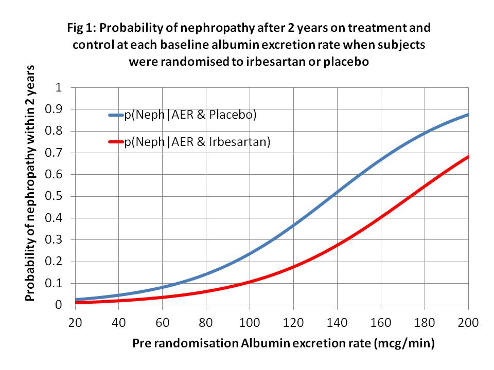
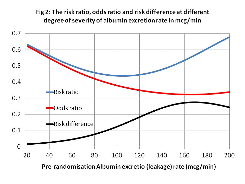
Looking at real example from Figure (1), let N = Y = nephropathy, Rx = x = treatment with irbesartan, A140 = z = an albumin excretion rate (AER) of 140mcg/min, when Pl = x’ = placebo and A40 = z’ = an AER of 40mcg/min. From Figure 1, p(N|Rx∩A140)rct = P(Y_x|z) = 0.24, p(N|Pl∩A140)rct = P(Y_x’|z) = 0.52 with a risk difference of 0.52-0.24 = 0.28. (The risk differences at various values of AER are shown in Figures 2 and 3.) There is a major benefit here from treatment when z = AER = of 140mcg/min so the patient will usually choose treatment after balancing with risks of adverse effects. Therefore the probability of nephropathy from this choice (i.e. p(Y|do(X=x),z) will be 0.52. (These are of course point estimates with no confidence limits at present).
When z’ = A40 = an albumin excretion rate (AER) of 40mcg/min, when Pl = x’ = placebo, from Figure 1, p(N|Rx∩A40)rct = P(Y_x|z’) = 0.02, p(N|Pl∩A40)rct = P(Y_x’|z’) = 0.04 with a risk difference of 0.04 – 0.02 = 0.02. There is little benefit from treatment when z’ = AER of 40mcg/min so it is not usually chosen. Therefore the probability of nephropathy from this choice (i.e. p(Y|do(X=x’),z’) will be 0.04.
When z’’ = A80 = an albumin excretion rate (AER) of 80mcg/min, from Figure 1, p(N|Pl∩A80)rct = P(Y_x’|z’’) = 0.14, p(N|Rx∩A80)rct = P(Y_x|z’’) = 0.04 with a risk difference of 0.14 – 0.06 = 0.08 as shown in Figure 3. There is little more benefit from treatment when z’’ = AER of 80mcg/min so some patients will choose treatment and some might not. Therefore the probability of nephropathy from a treatment choice (i.e. p(Y|do(X=x),z’’) will be 0.06 and from not choosing treatment it will be p(Y|do(X=x’),z) will be 0.14.
IF there was perfect consistency between an observation study, shared doctor/patient decision and RCT where P(Y|x,z)=P(Y|do[X=x],z)=P(Y_x|z) and P(Y|x’,z)=P(Y|do[X=x’],z)=P(Y_x’|z) then the fitting a logistic regression to plot of z against P(Y|x,z) and P(Y|x’,z) from an observation study might look like Figure 4. This could be regarded as a ‘pragmatic trial’ to assess the effectiveness of treatments when RCT results are put into practice. If the curves were indeed very similar to those of the RCT as shown by Figures 1 and 4, then this would suggest accurate probability estimates and treatment compliance. If the probability estimates shared with the patient by the doctor were poor, then the two curves might be shallower and if treatment compliance was also poor then they could be closer together.
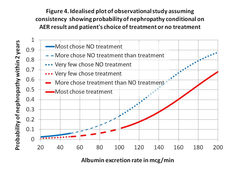
The interesting question here is whether the observation study in Figure 4 could be used in reverse to estimate the RCT result in Figure 1. For this to work well then the assumptions of P(Y|x,z)=P(Y|do[X=x],z)=P(Y_x|z) and P(Y|x’,z)=P(Y|do[X=x’],z)=P(Y_x’|z) have to be perfectly true. One important assumption is that choosing intervention or no intervention does not affect the processes that follow the choice to cause nephropathy. I suppose the validity of the assumption could be explored by doing RCTs first followed by ‘follow-up’ pragmatic trials. If the curves for treatment and no treatment from an observational study were different, then the observational study might provide evidence of effectiveness and minimum efficacy as the RCT might be assumed to display a larger difference.
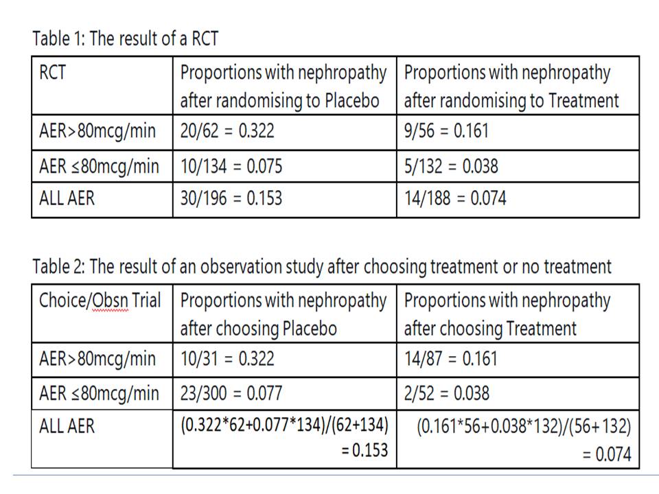
A similar exercise could be done by dichotomising the AER results (e.g. above or below an AER of 80mcg/min). Table 1 gives the results of the RCT. Table 2 gives the idealised observational study results of the choice arising from shared decision making. In this case a choice of placebo was made 31 times when the AER was over 80mcg/min and of these 10 were later found to have developed nephropathy giving a probability of 0.322, which is similar to the result for the RCT of 20/62 = 0.322. Again there were 300 individuals with an AER up to 80mcg/min. A decision was made to choose placebo in 300 and of these 23 developed nephropathy giving a probability of 0.077. In the RCT 10/134 = 0.075 developed nephropathy. These example data show how dichotomised results could also be used to conduct a pragmatic trial or perhaps to estimate the result of a RCT.
2 Likes
A question arising from my previous post is “Can a decisions to accept or reject a treatment be used sometimes as an instrumental variable when the conditions are right?”
The decision to tolerate possible adverse effects and take the treatment OR avoid them and refuse the treatment will depend on the doctor’s and patient’s personality and attitude to risk, the nature of the adverse and beneficial effects and the probabilities of the latter etc. The effect of nephropathy on well being and lifestyle could be assumed to be the same after taking treatment and after not taking treatment. For the same facts some will decide to opt for treatment and some will not.
Does the decision cause bias by affecting the way in which irbesartan reduces the risk of nephropathy? I cannot think of a mechanism that would cause this. I also cannot think of a mechanism why placebo should change the biochemistry either as the IRMA2 end point was biochemistry, not well being. Can anyone else? @f2harrell ? @Stephen ? @Pavlos_Msaouel ? @Martin_Dahlberg ? This is dependent on knowledge of the situation, which can never be complete of course (as in the case of Angrist and Imbens when using birth month as an instrument to assess duration of schooling on subsequent earnings).
A simple approach would be to suggest to the doctor and patient a theoretical lower risk of nephropathy of 10% on treatment when the ln(AER) is greater than 2 upper standard deviations of a healthy population, but a theoretical risk of side effects of 10% say on treatment. However, there is a higher theoretical risk of nephropathy of 20% on no treatment but without any risk of side effects. Based on the latter, please choose treatment or no treatment!
The real proportions with nephropathy for those on treatment and no treatment are then found by counting the number who actually developed nephropathy after 2 years in the treatment and no treatment groups. After 2 years, the proportions can also be found by an ‘observational study’ for each baseline AER as suggested by Figure 4 in the previous post. Unlike this example, an instrumental variable is only required when a RCT is not possible.
Many questionable assumptions are required when applying an instrumental variable compared to performing an RCT of course. Any comments?
3 Likes
Me neither. This is why I have been having such a hard time understanding the argument of the Mueller & Pearl paper that started this thread. Maintaining an open mind that perhaps I am missing something.
In our predictive modeling (technical example here and simplified description here) we have been distinguishing the estimation that informs inferences from the trade-offs that subsequently inform decisions. We do not do the opposite whereby the decisions are turned into inferences influencing estimations.
3 Likes
Counterfactual Prediction with counterfactual prediction evaluation!
Worth reading ![]()
Just reading the summary I wonder what is new there. And how did the authors account for bias in these observational treatment difference estimates?
Wouldn’t handling of treatment as a time-dependent covariate have been a simpler approach?
2 Likes
Are you familiar with Van-Geloven and Keogh approach for model evaluation under intervention?
This is the first time I’ve seen this approach being applied on a real case:
I’m specifically interested in counterfactual calibration on that context.
They’ve used the clone-censor-weight approach, there’s a nice part on the following youtube video (I’ve added a link to the specific point - 40:06) that demonstrates this approach.

I don’t know ![]()
But I can try and analyze an example they produced (regardless this specific article) with both approaches and see what will be the result ![]()
Prediction under an intervention the patient didn’t receive is just prediction, nothing really new. It’s just setting the treatment variable to the treatment of interest and getting predicted risks for all patients.
1 Like