Our Research Methods Program of the Vanderbilt Institute for Clinical and Translational Research and Vanderbilt Department of Biostatistics have created a fully sequential design and analysis plan for the COVID ordinal outcome scale that we’d like to share. Suggestions welcomed. It along with related resources may be found at http://hbiostat.org/proj/covid19 . The plan will be evolving, especially with inclusion of some Bayesian operating characteristic simulations. It is our hope that other academic groups and pharmaceutical companies may benefit from this plan. By allowing unlimited looks at the data with no need for conservative multiplicity adjustments (nor even a way to implement such adjustments) this design allows the most rapid learning about treatment effects.
I am curious about the data that goes into the model.
First, is the outcome for each patient the worst outcome experienced by the patient or the outcome on day 15 after randomization? I’d hope that some patients would improve (and therefore their ordinal outcome would increase in level) but would it be better to model whether a medication would have a better final outcome (at day 15) or less severe disease overall?
Second, the document states that the SOFA score is going to have a linear effect in the model. I may be mistaken but isn’t this a point-based score that could be broken up into a number of sub-scores or even the continuous underlying measurements? As a practical matter, is it required that all measurements be performed on the same day and how do multiple measurements come into play? For example, the bilirubin and CBC might be measured occasionally and the MAP measured continually. The ventilation status is a part of the SOFA score (as part of the respiratory status) but also part of the ordinal outcome (as outcome levels 2 and 3). Would it be the worst SOFA score in the day prior to randomization that would be used or the most recent score prior to randomization?
Overall, its really interesting to think about. Perhaps in the future an Excel spreadsheet could be provided for standardized data entry and then a Shiny app distributed for analysis as an R package. Stan models can be a bit compute-intensive to run on a public server but a virtual machine or Docker image might make it easier for those without R/Rcpp experience to use.
Great questions Eric.
I know of one study being planned that will measure the ordinal scale daily. For others I think it’s the status at day 14 regardless of the path to get there. I may be wrong.
Sample sizes are not large enough to allow for adjustment of individual SOFA components, I have not discussed with the critical care docs how the component measurements are made but I assume they are measured on the day of randomization.
Regarding data entry the best solution is REDCap and I am talking to our PIs about sharing the REDCap metadata/forms online.
At VUMC, if an IRB has been approved, then a REDCap project can be linked to Epic directly. This can allow pulling (some) data automagically from the EMR into REDCap and allowing other data to be updated from inside Epic/eStar to make it easier for clinicians and researchers to update patient’s information. It would also be possible to use the REDCap API to pull data directly into R and update an RMarkdown doc with the latest results (there may even be a way to use a web-hook to fire off recompiling the doc when changes happen to the REDCap data or just using a cron job.)
Alternatively, it shouldn’t be too difficult to put together some Epic Flowsheets, SmartTexts, and SmartLinks to pull the necessary data from the chart for use in documentation. VUMC eStar is currently on a build freeze pending the upgrade this weekend, but once that upgrade’s bugs get settled, this should be a straight-forward project for a physician builder of Epic analyst. Epic itself is even providing help to streamline the process (https://userweb.epic.com/Thread/96179/COVID-19-Clinical-Trials-Recruitment-Support/).
I’ll keep an eye out on the Epic forums for other Epic sites trying to do something similar. Most of what is up on the Epic userweb concerns ordersets for treating patients or dashboards to track testing and positive patients.
The main downside of this approach is that it while it could make it really easy for VUMC studies, it could be more difficult to translate to other institutions that don’t have REDCap.
I emailed @f2harrell some comments that are now posted at http://hbiostat.org/proj/covid19 . So, I guess it would be best for everyone to comment on the code in this thread.
Do people want me to amend the Stan code for the “basic ordered logit model” to do the thing where you put the Dirichlet prior on the conditional probability of falling in categories 1 … 7 for someone who has average predictors and then derive the cutpoints as transformed parameters from the inverse CDF of the logistic distribution?
I think that would be good, and anything you want to work on in the Bayesian proportional odds world would be helpful to many. As an aside I’m not a fan of the term “cutpoint” or the cutpoint notation but like to think this way (as in here:
Let the ordered unique values of Y be denoted by y_{1}, y_{2}, \dots, y_{k} and
let the intercepts associated with y_{1}, \dots, y_{k} be \alpha_{1}, \alpha_{2}, \dots, \alpha_{k}, where \alpha_{1} = \infty because \text{Prob}[Y \geq y_{1}] = 1. Let \alpha_{y} =
\alpha_{i}, i:y_{i}=y. Then
\text{Prob}[Y \geq y_{i} | X] = F(\alpha_{i} + X\beta) = F(\alpha_{y_{i}} + X\beta)
I don’t want derive cutpoints to be estimate intercepts. I know this is picky.
OK, I rewrote the Stan code to correspond to 13.3.1 of your PDF. The only differences are
- The lowest outcome category is 1 (as in the draft design) rather than 0 (as in the PDF)
- The Stan code assumes the design matrix has centered columns so that \alpha_j is the logit of \Pr\left(Y \geq j \mid \mathbf{x} = \mathbf{0}\right) for a person whose predictors are all average (even dummy variables).
This makes it possible to declare a simplex \mathbf{\pi} whose 7 elements can be interpreted as the probability of a person with average predictors falling into the corresponding outcome category. You can then put an uniformative Dirichlet prior on \mathbf{\pi} and derive \mathbf{\alpha} as an intermediate variable given \mathbf{\pi}.
However, the \boldsymbol{\alpha} in the Stan code are shifted by \overline{\mathbf{x}} \boldsymbol{\beta} relative to those in rms::orm where the predictors are not centered.
// Based on section 13.3.1 of http://hbiostat.org/doc/rms.pdf
functions { // can check these match rms::orm via rstan::expose_stan_functions
  // pointwise log-likelihood contributions
  vector pw_log_lik(vector alpha, vector beta, row_vector[] X, int[] y) {
    int N = size(X);
    vector[N] out;
    int k = max(y); // assumes all possible categories are observed
    for (n in 1:N) {
      real eta = X[n] * beta;
      int y_n = y[n];
      if (y_n == 1) out[n] = log1m_exp(-log1p_exp(-alpha[1] - eta));
      else if (y_n == k) out[n] = -log1p_exp(-alpha[k - 1]  - eta);
      else out[n] = log_diff_exp(-log1p_exp(-alpha[y_n - 1] - eta),
                                 -log1p_exp(-alpha[y_n]     - eta));
    }
    return out;
  }

  // Pr(y == j)
  matrix Pr(vector alpha, vector beta, row_vector[] X, int[] y) {
    int N = size(X);
    int k = max(y); // assumes all possible categories are observed
    matrix[N, k] out;
    for (n in 1:N) {
      real eta = X[n] * beta;
      out[n, 1] = log1m_exp(-log1p_exp(-alpha[1] - eta));
      out[n, k] = -log1p_exp(-alpha[k - 1]  - eta);
      for (y_n in 2:(k - 1))
        out[n, y_n] = log_diff_exp(-log1p_exp(-alpha[y_n - 1] - eta),
                                   -log1p_exp(-alpha[y_n]     - eta));
    }
    return exp(out);
  }
}
data {
  int<lower = 1> N;   // number of observations
  int<lower = 1> p;   // number of predictors
  row_vector[p] X[N]; // columnwise CENTERED predictors
  int<lower = 3> k;   // number of outcome categories (7)
  int<lower = 1, upper = k> y[N]; // outcome on 1 ... k

  // prior standard deviations
  vector<lower = 0>[p] sds;
}
parameters {
  vector[p] beta; // coefficients
  simplex[k] pi;  // category probabilities for a person w/ average predictors
}
transformed parameters {
  vector[k - 1] alpha;                               // intercepts
  vector[N] log_lik;                                 // log-likelihood pieces
  for (j in 2:k) alpha[j - 1] = logit(sum(pi[j:k])); // predictors are CENTERED
  log_lik = pw_log_lik(alpha, beta, X, y);
}
model {
  target += log_lik;
  target += normal_lpdf(beta | 0, sds);
  // implicit: pi ~ dirichlet(ones)
}
generated quantities {
  vector[p] OR = exp(beta);
}
This looks great @bgoodri! I have a development version of a package which implements a closely related Stan model on github here. The goal of this package/code is to analyze continuous or mixed continuous/discrete outcomes using cumulative probability models (i.e., the number of outcome categories k is similar or equal to the number of observations n). One big difference is the concentration parameter for the Dirichlet prior on \pi. Since we only have a small number of observations in each category, using the usual uninformative symmetric Dirichlet doesn’t work very well. Currently the package uses a concentration parameter of 1/k based on a heuristic argument that this is equivalent to adding 1 pseudo-observation, but I’m exploring other options.
Where in this design would substantive theories of postulated therapeutic effects enter into consideration? Take for example the several theories advanced in [1,pp5–6]:
Findings from previous studies have suggested that chloroquine and hydroxychloroquine may inhibit the coronavirus through a series of steps. Firstly, the drugs can change the pH at the surface of the cell membrane and thus, inhibit the fusion of the virus to the cell membrane. It can also inhibit nucleic acid replication, glycosylation of viral proteins, virus assembly, new virus particle transport, virus release and other process to achieve its antiviral effects.
… and then later on pp.15–16:
In some patients it has been reported that their immune response to the SARS-CoV-2 virus results in the increase of cytokines IL-6 and IL-10. This may progress to a cytokine storm, followed by multi-organ failure and potentially death. Both hydroxychloroquine and chloroquine have immunomodulatory effects and can suppress the increase of immune factors[29, 30]. Bearing this in mind, it is possible that early treatment with either of the drugs may help prevent the progression of the disease to a critical, life-threatening state.
How would continuous learning proceed about the several mechanisms of action posited here? I have to think that incorporating more information via multivariate, time-series outcomes would be essential. As I read it, the design in its present form seems organized around a single, ordinal outcome measure as its central feature.
- Yao X, Ye F, Zhang M, et al. In Vitro Antiviral Activity and Projection of Optimized Dosing Design of Hydroxychloroquine for the Treatment of Severe Acute Respiratory Syndrome Coronavirus 2 (SARS-CoV-2). Clinical Infectious Diseases. March 2020:ciaa237. doi:10.1093/cid/ciaa237
ADDENDUM:
A March 23 paper [2] came to my attention this morning, which illustrates some of the opportunities for obtaining quantitative time-series data on the course of illness. N=23 patients were followed serially, with a mean of 7.5 respiratory specimens on which reverse transcriptase quantitative PCR (RT-qPCR) was done to quantify SARS-CoV-2 RNA. Moreover, serology for IgG and IgM antibodies to the virus surface spike receptor binding domain (RBD) and internal nucleoprotein (NP) were used to (semi?)quantitate antibody responses. The paper claimed, e.g., that initial viral load was high initially, and declined steadily. This suggests an opportunity to model the slope of log10 copies/mL RNA—a chance to estimate rather than hypothesis-test, which should please some of you! Furthermore, the onset of antibody response offers up a time-to-event outcome that might be worth modeling. (But on that latter point, please note that the IgG response and its timing may have a subtler—spline-able?—relation to outcomes as discussed at the top left-hand column on p.9 including with correlation to macaque experimental studies. This thread by virologist Akiko Iwasaki has a nice further explanation of the point made there.)
- To KK-W, Tsang OT-Y, Leung W-S, et al. Temporal profiles of viral load in posterior oropharyngeal saliva samples and serum antibody responses during infection by SARS-CoV-2: an observational cohort study. The Lancet Infectious Diseases. March 2020:S1473309920301961. doi:10.1016/S1473-3099(20)30196-1
@bgoodri and @ntjames we’re having a new challenge where we may need a special longitudinal ordinal model that handles an absorbing state (death). This approach has promise. Would you want to take a crack at, or recommending someone good at Stan model coding, implementing this state transition proportional odds model? I’m happy to only have this for the p=1 case (first order Markov model).
Adding a patient-specific shift — as suggested in the draft — would be easy. Adding Markovian dynamics — as suggested in your reply — is possible but much more involved.
The Lee and Daniels paper that you linked to is essentially a discrete ordinal state, discrete time Markov model. That could be appropriate if the patient’s state were reevaluated hourly or some regular interval like that, but it sounds as if (someone who is talking to) you might be envisioning a discrete state, continuous time Markov model where at each instant a live patient has a high chance of staying in the same state but a slight chance of moving to a better or worse state. That would be more appropriate if the time intervals are implicitly defined as whenever there is a change in state for the patient. In other words, would the data be recorded like
- Patient n was admitted to the hospital in state 5 with these covariates \dots
- Patient n randomized into the control group 32 minutes later
- Patient n was downgraded to state 4 after 1 day, 2 hours and 16 minutes
\dots
?
In addition to the absorbing state of death, we presumably have to incorporate the restriction that the patient has to be alive at the time the randomization into treatment or control takes place. Also, it seems like there might be some restrictions where a patient cannot jump across too many states at once. As in, is it realistic for someone to go from state 5 to state 2 without passing through states 4 and / or 3?
Thanks for these thoughts Ben. I’m recording a discussion related to some of these points, where co-author Mike Daniels is involved in the discussion. Mike responded this morning that there is no restriction as to the number of categories that can be jumped in one time period.
There are three setups for this problem, as you alluded to:
- The simplest in which ordinal outcomes are measured daily for a set length of time, say 14 days, or until the aborbing state is hit (death)
- Similar to the first but where measurements are not equally spaced, e.g. scheduled assessments at baseline, day 1, day 3, day 7, day 10, day 14.
- The more general case where the last assessment may be distant from the others or different types of patients would be assessed at different times.
Ultimately it would be good to handle all 3 situations but priority for now is for the first and second.
Nathan does Stan automatically center covariates behind the scene when using your package, and do the “secretly translate back to the original data” for you?
No, for now it is similar to the code that Ben shared above. The calculation of the cumulative probabilities is anchored to \boldsymbol{x=0}. If the covariates are not centered by the user, the model may extrapolate outside the observed range of the data.
Can I get some opinions on the ordinal longitudinal model in section 2.1 of
It seems fairly similar to the article by Lee and Daniels that @f2harrell mentioned but a bit easier to implement.
Dear Dr. Harrell and Co.,
Thank you for posting this RCT design. I have been working through it to inform RCTs I am designing (and would like to design in the future) and I had the following questions as I have worked through the code.
-
Am I correct that the non-uniform priors you are comparing against the flat in this modeling are measures of how much one believes the OR=1?
-
As my intuition is still limited, the first two plots (Look vs Mean Reduction) and (True OR vs Median Lag) don’t seem super informative, as the Prior P(OR>2) are arbitrary (OR>k where k really could be anything…?). How do these plots help in design and execution of the trial (esp. regarding when it is ok to stop?) Also, I have not been able to understand yet why Fig. 2 is concave, i.e. why the median lag for Prior P=0.01 is the same for True OR = 1.5 and True OR ~= 1.8?
-
If I do have prior information, is the best way to encode it is in mean.prior=log(OR_prior), and then cut.prior=log(OR_prior+k ) (where k>0)? When I do this is it seems to mess up to the lag calculations for Fig. 1 and Fig. 2…
-
This is less of a conceptual problem and more of a specific case problem: Frustratingly enough, the case I am considering (reduced LOS) results in OR<1, where here your code seems set up for OR>1. Is there a simple way to flip the code, (say, setting the simulation (simdat) ORs to be 1/OR so that the rest of the prior calculations are unharmed,) or do I need to go through and flip all the signs?
I appreciate any time anyone can provide to help me untangle these issues for me.
Best,
Alan
You’re welcome.
yes
The choice of k is a bit arbitrary but I still think reasonable. These plots are more to study the prooperties and likely outcomes of the sequential trial than to assist in interpreting results. But I’m going to update the document tonight to clarify that you should probably use different priors for different types of assessments, e.g., I lean to a flat prior to getting evidence for non-efficacy or similarity. Sorry I don’t have time to deal with the last part of that question.
If you can approximate your prior with a normal distribution in the log odds ratio it’s best to modify the code to use a non-zero mean for the prior, and to insert the variance of the prior, both in the calls to gbayes (and maybe elsewhere).
You can flip a lot of it, or just modify the code. For our case, larger Y is better (not typical). I can post tne entire Rmarkdown file if needed.
Dear Dr. Harrell and Co.
Thank you for the replies. I have been continuing to work through the code and I believe I have found some typos in what is posted. Please let me know if there is a better venue in which to post them:
In the code block before Figure 3.
Line 7:
f <- lrm(y ~ rcs(log(or), 5), data=d, maxit=30)
Should be
f <- lrm(y ~ rcs(log(ors), 5), data=d, maxit=30)
I think, otherwise rcs has two scalars as its two arguments.
Line 16
for(ty in types) {
Should be
for(ty in numtypes) {
As “types” will generate objects like “similarity” but data frame R has integers in its “type” column
Thank you again for your time.
-Alan
Another typo and question
In the code before Figure 4, I believe
Line 18
for(ty in types) {
Should be
for(ty in numtypes) {
As “types” will generate objects like “similarity” but data frame R has integers in its “type” column
Separately, when I run the code for Figure 4, for the first panel I get
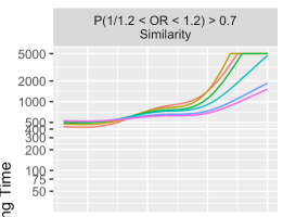
rather than the behavior in your Figure 4, where the PriorP 0.499 and 0.25 sharply increase to 5000 at ~ 1.75, which is more in line with the other panels where the plotted behavior changes gradually from 0.499 -> 0.25 -> 0.1 -> 0.05 -> etc
Thank you again for this tremendous resource.
- Alan
Please check again. The dataset d being analyzed by lrm is a subset of R which has the variable or not the variable ors in it. And rcs takes a vector and either a scaler (# knots) or vector (knot locations).
Please check again. R was loaded from simlooks and before simlooks was stored it converted R to a data frame and made type a character variable.
Please check again. Similar comment as above. The code looks out of order but it’s because I run it once to compute slow things, then set a “done” type of variable to TRUE so that the results can be loaded back. I usually use cache=TRUE to do all this but sometimes I like more control, or smaller cache.
I do appreciate your checking the code carefully as you have done. Another pair of eyes is always important.