I am trying to wrap my head around methodological issues while constructing a predictive model.
The predictive model was developed following the Tripod guidelines. It has a defined use-case. An ordinal logistic regression model was chosen and the outcome variable defined based on subject matter knowledge of clinical collaberators without “looking at the data”. The included covariates where chosen based on subject matter knowledge, and respecting the number of candidate parameters the data could support.
Now I have fit a tentative ordinal model. Examining the residuals, there are some covariates which show strong evidence of not following the proportional odds assumption. However, most of the variables are binary, 0 and 1 which I feel may affect the interpretation of the importance of this violation. I am also aware that there is a literature regarding the proportional hazards assumption, and that violations of this may not matter. I am therefore curious how I should proceed, when I have already chosen the model and the variables, but now find violations.
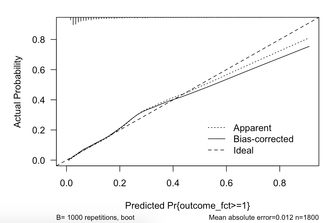
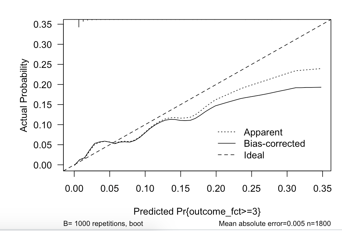
Specifically when I do not believe the violations have any real significance to the model performance. Here I show the calibration plots for the first, second and third outcomes. The third outcome is rare, and I am not surprsied it performs relatively poorly. The overall model seems to perform well. How to I reconcile violations of assumptions with this fact?
This is a really excellent question and one that comes up often, but the literature on what to do about non-proportional odds for a minority of predictors is not fully developed. Here are some random thoughts:
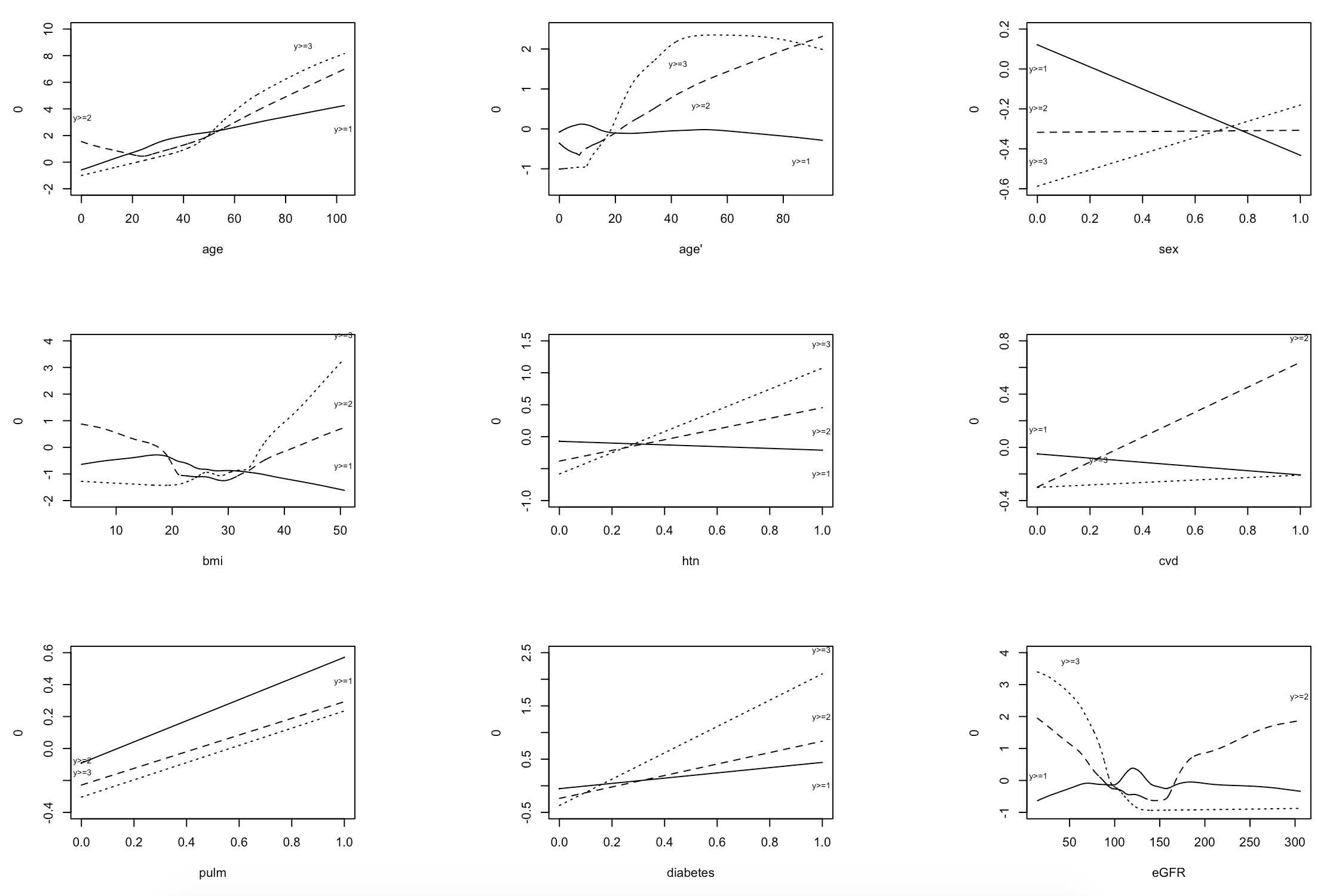
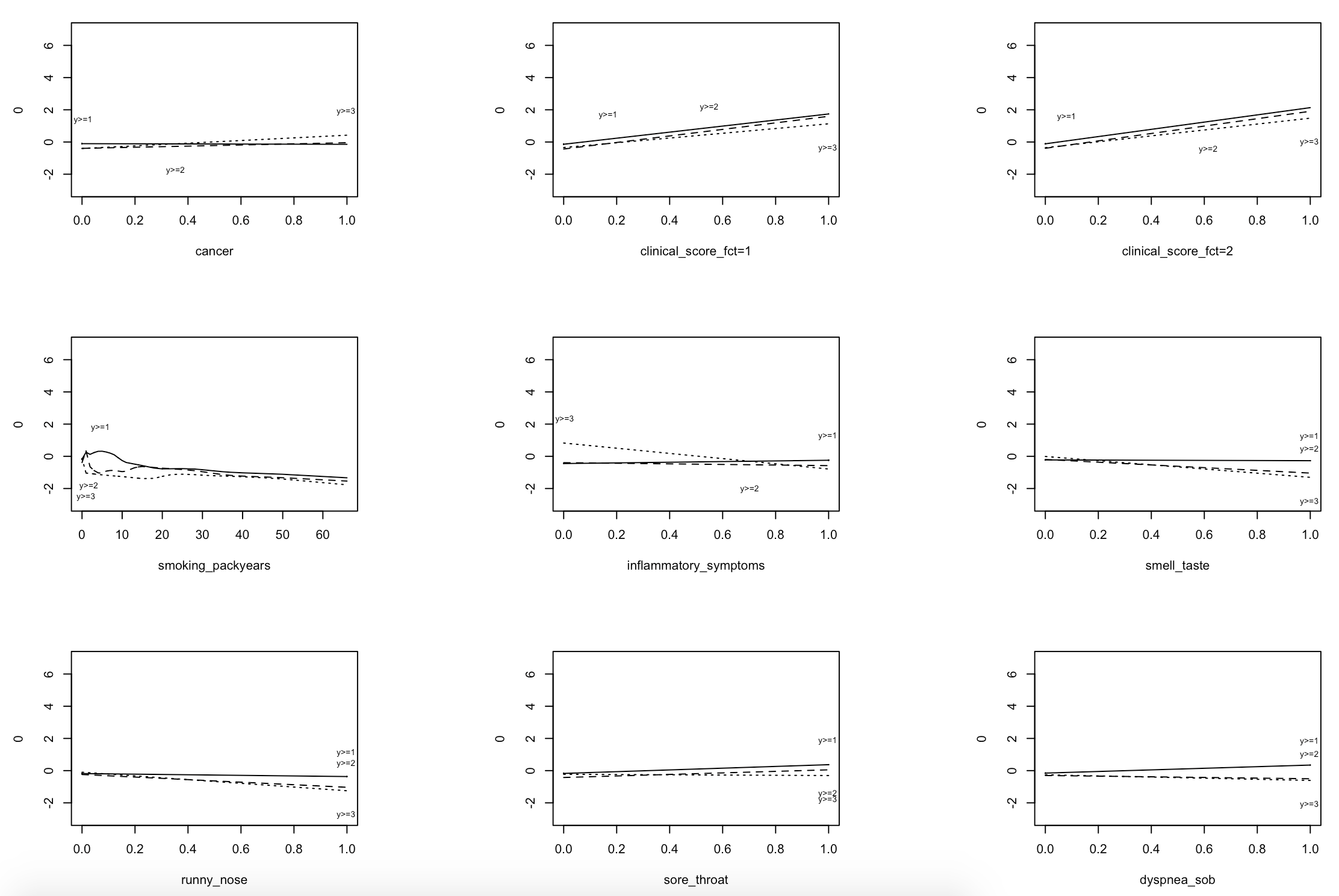
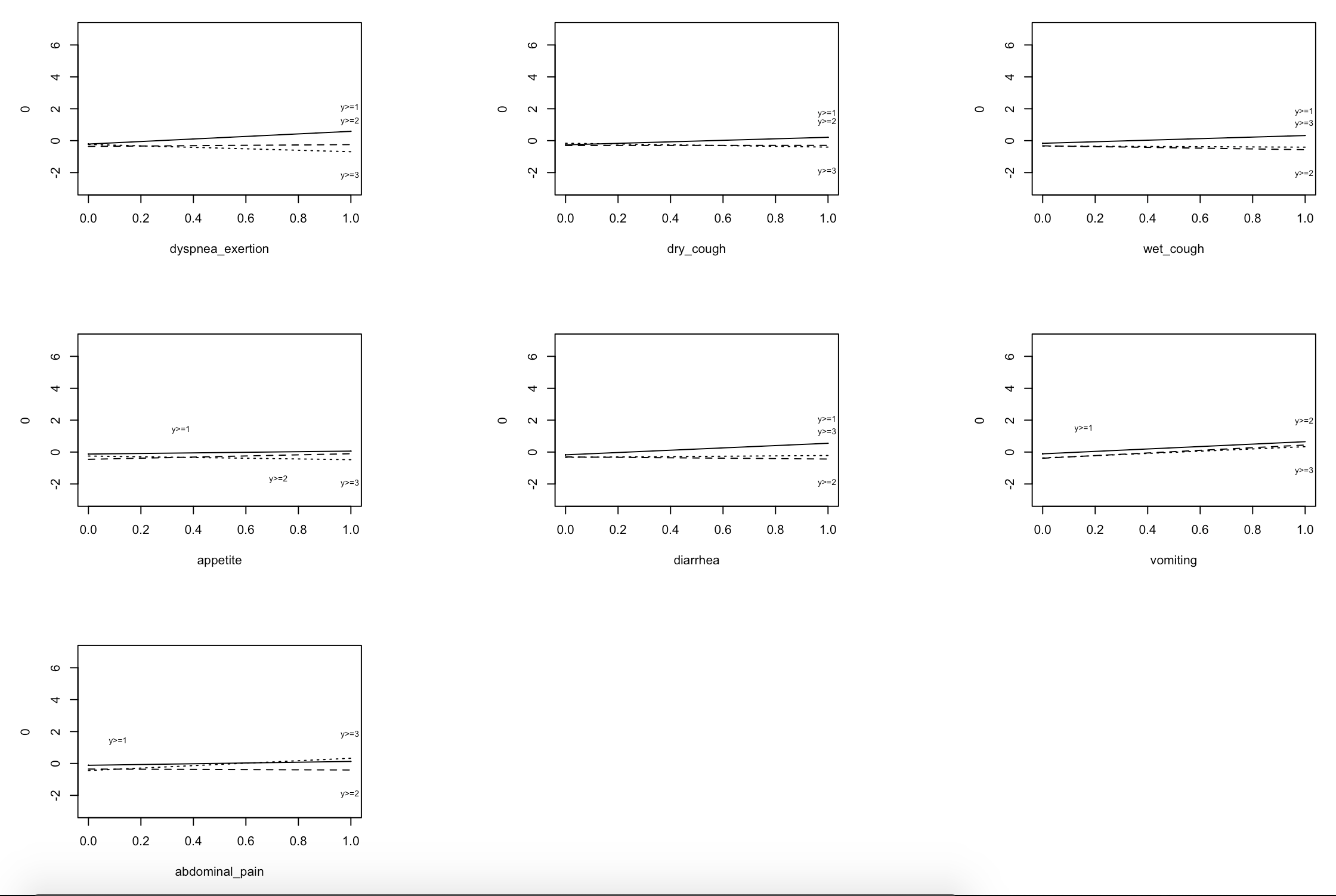
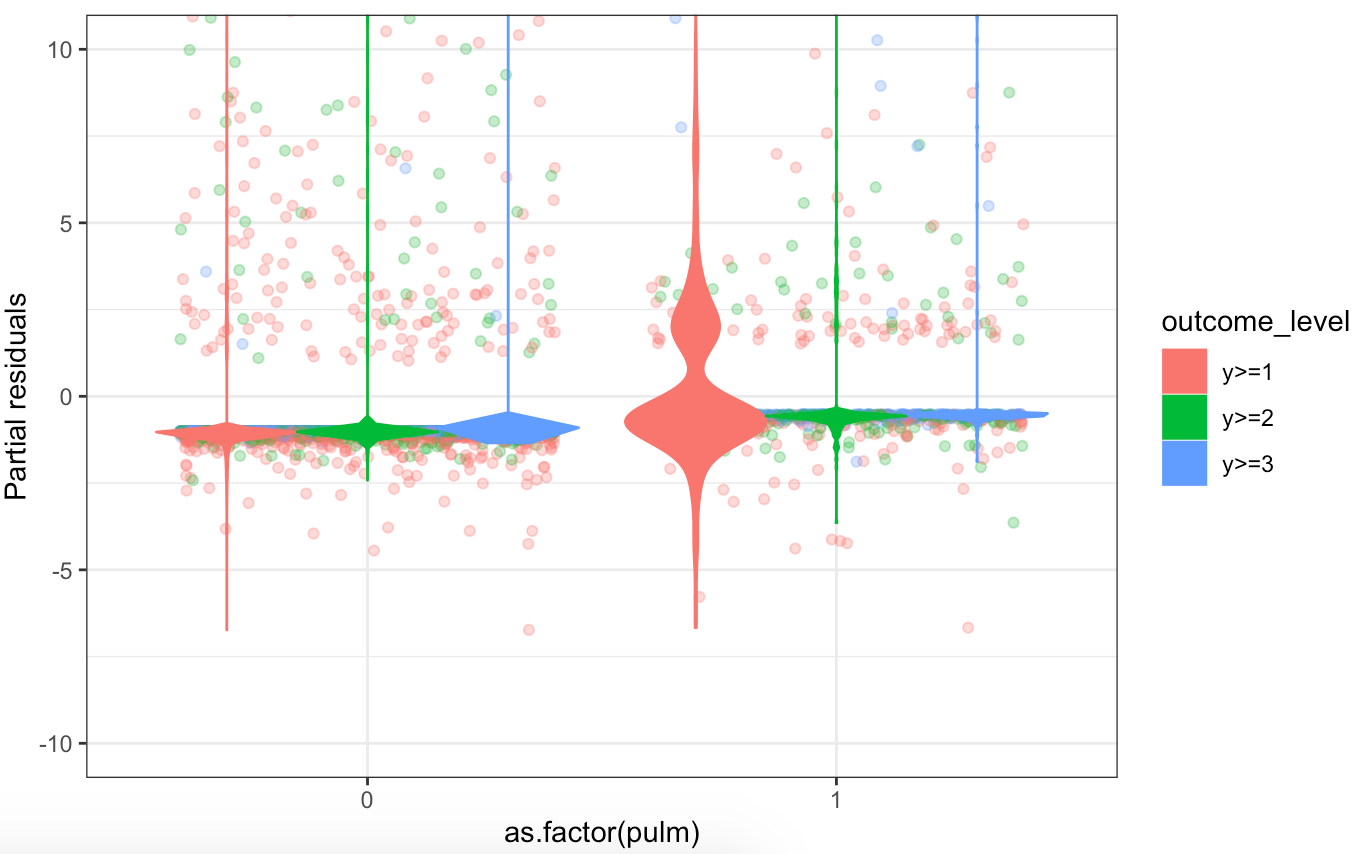
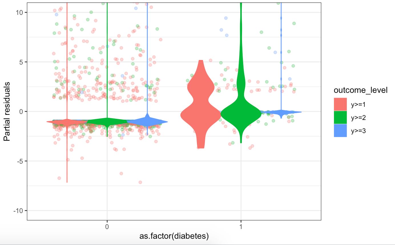
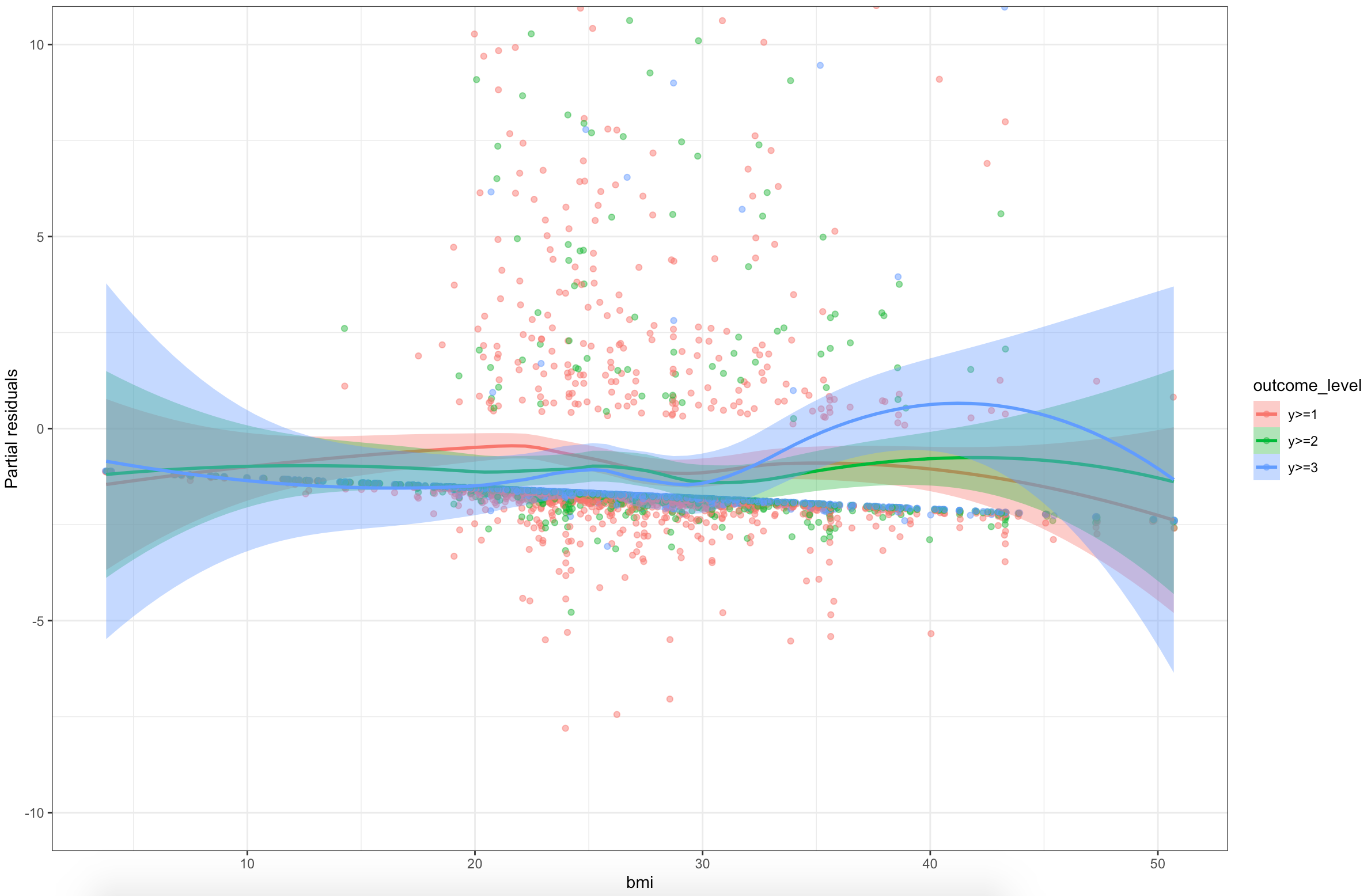
The partial residual plots need to be put on a common scale and interpreted in such a way that non-PO in minor predictors is de-emphasized
Fitting a model that has non-PO for a minority of predictors is almost always better than alternative models which may have different assumptions violated, and is certainly better than fitting separate binary logistic models
The most rational approach, though one that complicates the model, is to use a Bayesian partial proportional odds model where priors are put on model components that represent departures from PO. In other words we have somewhat skeptical priors on the extra model terms that favor PO but allow for non-PO as the sample size expands and more information is available for such customization (just as as do for Bayesian modeling of covariate interactions). This is implemented in the new R rmsb package which will be available on CRAN on about 2020-07-23 and for which many examples are shown here.
Thank you for your reply! I would love to better understand the interpretation of residuals in binary logistic and ordinal logistic models. I have been using your excellent RMS book (and course, and package).
[quote="f2harrell, post:2, topic:3585]
The partial residual plots need to be put on a common scale and interpreted in such a way that non-PO in minor predictors is de-emphasized
[/quote]
Showing the partial residuals on a common scale definitely does drive home the point how minor these violations are for most variables.
I still wonder what effect (if any) the dichotomous nature of the variables have on the interpretation of ordinality. The above approach seems to assume that the variable is continuous. I played around with visualisations, but I imagine I am just misunderstanding the problem at hand.
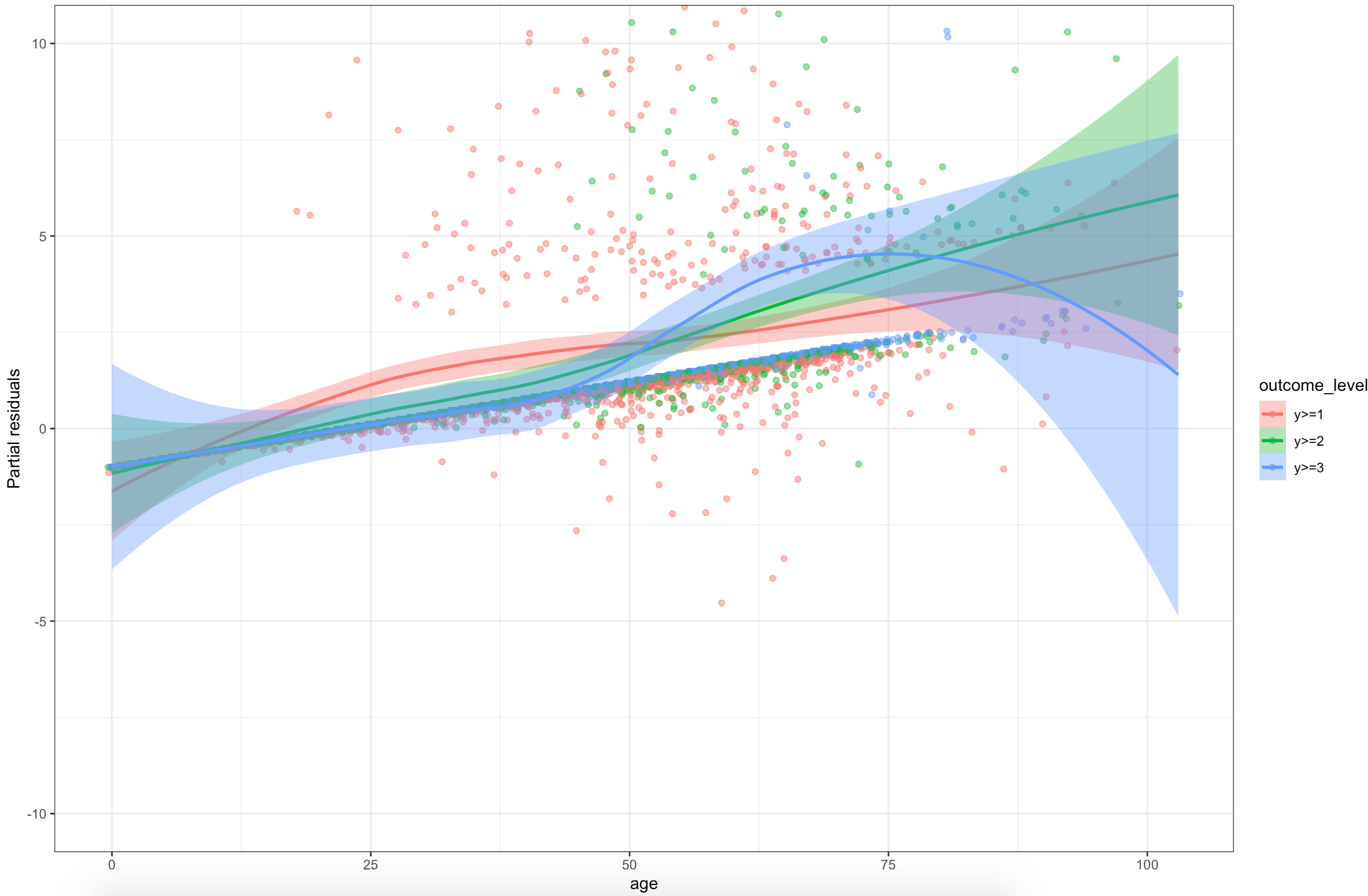
Likewise, I wonder if confidence limits to the LOESS smoother for the partial residuals aids in interpretation of the seriousness of the ordinality violation. I notice that the LOESS trend tends to diverge where there is the lease amount of information in the data. Again, this could all just be a big misunderstanding on my part.
Yet another reminder that I have to push for clinical time off to finish Richard McElreath’s book to get started on understanding Bayesian approaches. The package looks amazing.
And if the failing variable is a non-linear continuous variable, eg a spline, what is best to do? A PPO model without proportionality for the spline, or a PO model ignoring the issue?
Sometimes you find that a different link function works better, but then you have trouble interpreting the effects. I would go usually with the constrained partial proportional odds model. Example of the Bayesian Wilcoxon test is in the link above, where the departure from proportional odds is linear in transformed y. It should be on CRAN in 2 days, and requires a new version of the rms package also, which is already on CRAN.
I have been reading about the constrained partial proportional odds model, and thought it was beautiful. But, in that case, is it a good idea to use the proportionality constraints for the spline coefficients of continuous variables? These coefficients usually violate the assumption of PO the most. In principle, it should be possible, as with other variables, right?
And, can you explain the interpretation of the coefficientes from the Constrained Partial Proportional Odds Ordinal Logistic Model??
For example, the response variable h7 has 3 ordered levels (poor, regular, good) and cir is a binary predictor (0,1).
Constrained Partial Proportional Odds Ordinal Logistic Model

 blrm(formula = h7 ~ cir, ppo = ~cir, cppo = function(y) y ==
     "good", data = DAT)

                    Mixed Calibration/             Discrimination                Rank Discrim.
                Discrimination Indexes                    Indexes                      Indexes
     Obs219    LOO log L-194.75+/-9.02    g  0.348 [0.001, 0.708]    C    0.617 [0.366, 0.634]
      poorl21     LOO IC   389.5+/-18.04    gp      0.03 [0, 0.063]    Dxy 0.234 [-0.269, 0.269]
  regular63     Effective p4.02+/-0.35    EV     0.014 [0, 0.042]
   good135     B 0.087 [0.086, 0.088]    v      0.168 [0, 0.511]
  Draws4000                               vp     0.001 [0, 0.004]
    Chains4
     p    1

              Mode Beta Mean Beta Median Beta S.E.   Lower   Upper   Pr(Beta>0) Symmetry
 y>=regular    2.5648    2.5896    2.5731     0.3471  1.8988  3.2595 1.0000     1.16
 y>=good       0.7290    0.7217    0.7184     0.1905  0.3650  1.0949 1.0000     1.06
 cir=1        -0.6076   -0.6111   -0.6069     0.2964 -1.1675 -0.0187 0.0163     0.93
 cir=1 x f(y)  0.0375    0.0376    0.0357     0.2136 -0.3693  0.4637 0.5692     1.05
So, in order to understand cir=1 x f(y) I need to manually obtain the beta coefficient for regular and good?
I have seen this in the vignette but how can I calculate that myself?
h <- bs22$cppo
k <- coef(bs22)
k
k[3] + h(1:2) * k[4]
So glad to see the new rmsb package used Alberto. You are close. Before answering your question directly you can use Predict(fit, ycut='regular') or contrast(fit, list(...), list(...), y=c('regular', 'good')). For the manual approach, use e.g.
k <- coef(fit, 'mean')   # if using posterior mean parameters
k['cir=1']   # beta coefficient for y >= 'regular'
k['cir=1'] + k['cir=1 x f(y)'] * cppo('good')     # beta for y = 'good'
Well, I’m glad you’re glad, I have been using your codes for years, but now I have a lot of doubts on this model… For example, this is the output from constrast, but to understand the Peterson-Harrell model I would like to know the interpretation of cir=1 x f(y) 0.0375 above. For example:
> contrast(bs22, list(cir=1), list(cir=0), y=c("good","regular","poor"))
                 Contrast      S.E.     Lower       Upper Pr(Contrast>0)      NA
1   h7=good -0.5814817 0.2799829 -1.116538 -0.03558248         0.0135    bien
2   h7=regular -0.6586901 0.4706123 -1.598199  0.23096145         0.0755 regular
3*  h7=poor -0.6586901 0.4706123 -1.598199  0.23096145         0.0755     mal

Redundant contrasts are denoted by *

Intervals are 0.95 highest posterior density intervals
Contrast is the posterior mean
I suppose the output above are log odd ratios but how can I derive the -0.58 from the model coefficients?
Also I don’t understand the difference between the estimates from contrast and this:
k <- coef(bs22, 'mean')   # if using posterior mean parameters
k['cir=1']   # beta coefficient for y >= 'regular'
     cir=1
-0.6110959
Something seems to happen with cppo, R tell me that the function can’t be found:
> k['cir=1'] + k['cir=1 x f(y)'] * cppo('good')     # beta for y = 'good'
Error in cppo("good") : no se pudo encontrar la función "cppo"
Also can you please explain the interpretation of this??
Thank you, Frank, if cir=1 is radical mastectomy and cir=0 is breast conserving surgery, and hr7 is quality of life at the end of chemotherapy, can you help me interpret these coefficients, please? In particular, I have been reading Peterson & Harrell 1990, and I understand Eq. 6 for the constrained model as β + Γ*γ but I don’ t understand the reason to normalize gamma Γ by the weighted mean and sd of Y (in this case it is quality of life).
The normalization of the \Gamma function (called cppo in blrm) is done to make MCMC behave better in the Bayesian posterior sampling. Always use the derived cppo function from the fit object in all of your calculations and you can ignore that this is happening, since the modified cppo function does the scaling and centering automatically.
But if you normalize, the beta coefficient changes as well. For example, in the cisplatin example, in the blrm output, the beta is 0.94, but after applying the cppo formula the final result is 1.06.
Likewise, I can no longer interpret γ as the factor by which 0.94 varies for Y=5…
Also what happens if you can’t predict the coefficients linearly?
I’m not getting your question. As long as you always multiply the regression coefficient by fit$cppo(y) you’ll have the right answer. When communicating to others just print the function so they can incorporate the same scale/centering.
I understand that you mean that the model estimates are invariant after normalization, and this does not affect the predictions either. I think I’m going to start a new thread in datamethods for practical or code issues with the new package, with your permission. It will be easier for other people to find in google. Thanks.